Motivation of canonical correlation analysis (CCA)

The main motivation of CCA is to provide multi-view of the data, which usually consists of two sets of variables. Canonical correlation analysis determines a set of canonical variates, i.e., orthogonal linear combinations of the variables within each set that best explain the variability both within and between sets. So there could be multiple dimensions (canonical variables) that represent the association between two sets of variables. That yields multiple aspects, aka, multi-view, for the data.

Problem setup

For $n$ observations, there are two sets of variables observed, denote as $X \in R^{n \times p_{1}}$ and $Y \in R^{n \times p_{2}}$ . We hope to find out a combination of variables in $X$ , denoted as $X u$ , and a combination of variables in $Y$ , denoted as $Y v$ such that maximize their correlation. This $(X u, Y v)$ is called the first canonical pair. The objective of CCA is thus $max_{u, v} corr (X u, Y v)$ Assuming $X$ and $Y$ are centered, then the objective function can be written as $\begin{matrix} (1) & max_{u, v} \frac{Cov (X u, Y v)}{(Var (X u) Var (Y v))^{- 1 / 2}} = \frac{u^{T} Σ_{X Y} v}{\sqrt{u^{T} Σ_{X} u v^{T} Σ_{Y} v}} \end{matrix}$ where $Σ_{X Y} = E (X^{T} Y), Σ_{X} = E (X^{T} X), Σ_{Y} = E (Y^{T} Y)$ .

The objective (1) is equivalent to $\begin{aligned} max_{u, v} & u^{T} Σ_{X Y} v \\ s.t. & u^{T} Σ_{X} u = 1 \\ v^{T} Σ_{Y} v = 1 \end{aligned}$ which is a very standard optimization problem.

Here we propose a common strategy in solving optimization problem (1). Denote $\tilde{u} = Σ_{X}^{1 / 2} u$ and $\tilde{v} = Σ_{Y}^{1 / 2} v$ , then we obtain $\begin{matrix} (2) & max_{\tilde{u}, \tilde{v}} \frac{{\tilde{u}}^{T} Σ_{X}^{- 1 / 2} Σ_{X Y} Σ_{Y}^{- 1 / 2} v}{\sqrt{{\tilde{u}}^{T} \tilde{u} {\tilde{v}}^{T} \tilde{v}}} \end{matrix}$ Recall the objective function of PCA (for the principal component) $max_{u} \frac{u^{T} X^{T} X u}{u^{T} u}$ which shares the similar structure and could be solved by eigendecomposition. Following the same logic, as $u$ and $v$ are of different length, problem (2) could be solved by SVD. Denote the SVD of $Σ_{X}^{- 1 / 2} Σ_{X Y} Σ_{Y}^{- 1 / 2} = P Λ Q^{T}$ , the solution of $(\tilde{u}, \tilde{v})$ is $(P_{1}, Q_{1})$ corresponding to the largest singular value. Thus, we obtain $(u, v) = (Σ_{X}^{- 1 / 2} P_{1}, Σ_{Y}^{- 1 / 2} Q_{1})$ .

Extending to multiple canonical pair $(u_{i}, v_{i}), i = 1, . . ., min (p_{1}, p_{2})$ , denote them in the matrix form as $(U, V) \in (R^{p_{1} \times min (p_{1}, p_{2})}, R^{p_{2} \times min (p_{1}, p_{2})})$ . The solution is, with the same logic, $\begin{matrix} (3) & (U, V) = (Σ_{X}^{- 1 / 2} P, Σ_{Y}^{- 1 / 2} Q) \end{matrix}$

Usually we only need the first several canonical pairs to view the data. So CCA is basically another way to accomplish dimension reduction.

Toy example

Let’s check it with a toy example:
A researcher has collected data on three psychological variables, four academic variables (standardized test scores) and gender for 600 college freshman. She is interested in how the set of psychological variables relates to the academic variables and gender. In particular, the researcher is interested in how many dimensions (canonical variables) are necessary to understand the association between the two sets of variables. (ref)

First, we use the existing R package CCA to conduct the analysis.

mm <- read.csv("https://stats.idre.ucla.edu/stat/data/mmreg.csv")
colnames(mm) <- c("Control", "Concept", "Motivation", "Read", "Write", "Math", "Science", "Sex")
# i.e. X: 600x3; Y: 600x5

psych <- mm[, 1:3]
acad <- mm[, 4:8]
cc1 <- cc(psych, acad)
round(cc1$xcoef,4) # i.e. U: 3xmin(3,5)

##               [,1]    [,2]    [,3]
## Control    -1.2538 -0.6215 -0.6617
## Concept     0.3513 -1.1877  0.8267
## Motivation -1.2624  2.0273  2.0002

round(cc1$ycoef,4) # i.e. V: 5xmin(3,5)

##            [,1]    [,2]    [,3]
## Read    -0.0446 -0.0049  0.0214
## Write   -0.0359  0.0421  0.0913
## Math    -0.0234  0.0042  0.0094
## Science -0.0050 -0.0852 -0.1098
## Sex     -0.6321  1.0846 -1.7946

cc1$cor # canonical correlations

## [1] 0.4640861 0.1675092 0.1039911

We can also do it manually using the expression in (3).

# do it manually
mm = apply(mm, 2, function(x) scale(x, center = T, scale = F))
psych <- mm[, 1:3]
acad <- mm[, 4:8]
Sig_x = t(psych)%*%as.matrix(psych); Sig_xsqrt = sqrtm(Sig_x)
Sig_y = t(acad)%*%as.matrix(acad);   Sig_ysqrt = sqrtm(Sig_y)
Sig_xy= t(psych)%*%as.matrix(acad)
MM = solve(Sig_xsqrt)%*%Sig_xy%*%solve(Sig_ysqrt)
res = svd(MM)
res$d ## which is just cc1$cor

## [1] 0.4640861 0.1675092 0.1039911

solve(Sig_xsqrt)%*%res$u # U

##             [,1]        [,2]        [,3]
## [1,] -0.05123026 -0.02539288 -0.02703590
## [2,]  0.01435577 -0.04852756  0.03377890
## [3,] -0.05158110  0.08283177  0.08172711

solve(Sig_ysqrt)%*%res$v # V

##               [,1]          [,2]          [,3]
## [1,] -0.0018231483 -0.0002006181  0.0008735867
## [2,] -0.0014658991  0.0017189940  0.0037307163
## [3,] -0.0009568002  0.0001728118  0.0003839993
## [4,] -0.0002053221 -0.0034796325 -0.0044877370
## [5,] -0.0258276917  0.0443172840 -0.0733272900

Notice that the results are the same to that from the package, except there is a scale difference.

We can construct the first canonical pair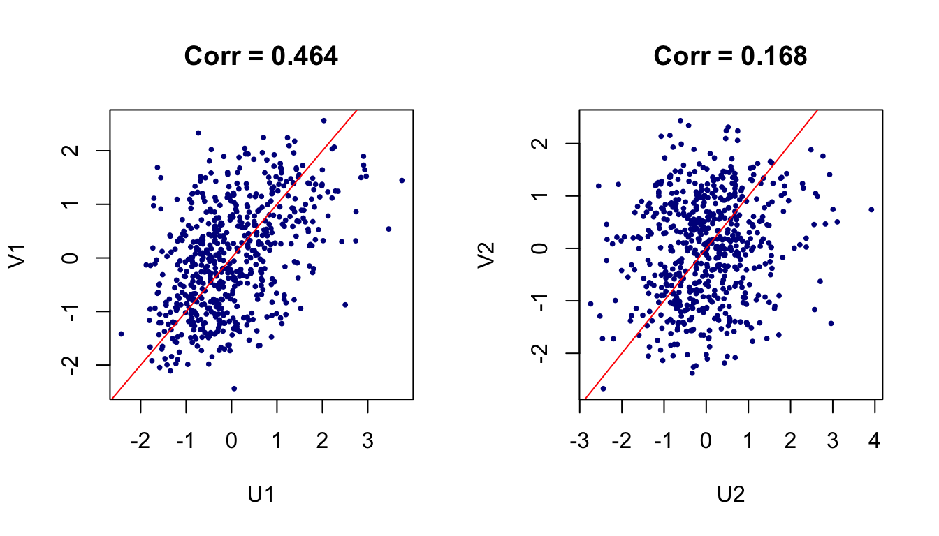

(u_{1}, v_{1}) = (- 1.25 C o n t r o l + 0.35 C o n c e p t - 1.26 M o t i v a t i o n, - 0.045 R e a d - 0.036 W r i t e - 0.023 M a t h - 0.005 S c i e n c e - 0.632 [f e m a l e = 1])

. Similarly, we can construct

(u_{2}, v_{2})

. The original data can thus be viewed from canonical pairs, as shown in figure below.

Figure 1: Viewing data on the first two canonical pairs.

Regularized CCA

For high dimensional data, it is more desirable to incorporate sparsity to construct canonical pairs using limited number of covariates. It helps to have a more clear picture of the results. Generally, we can add penalty terms to the objective function to accomplish this task, such as ridge penalty $\begin{aligned} max_{u, v} & u^{T} Σ_{X Y} v - λ_{1} | | u | |_{2} - λ_{2} | | v | |_{2} \\ s.t. & u^{T} Σ_{X} u = 1 \\ v^{T} Σ_{Y} v = 1 \\ λ_{1}, λ_{2} \geq 0 \end{aligned}$

which is equivalent to $\begin{aligned} max_{u, v} & u^{T} Σ_{X Y} v \\ s.t. & u^{T} (Σ_{X} + λ_{1} I) u = 1 \\ v^{T} (Σ_{Y} + λ_{2} I) v = 1 \\ λ_{1}, λ_{2} \geq 0 \end{aligned}$ or $max_{u, v} \frac{u^{T} Σ_{X Y} v}{\sqrt{u^{T} (Σ_{X} + λ_{1} I) u v^{T} (Σ_{Y} + λ_{2} I) v}}$ which could be solved nearly the same as CCA.

Subgroup Identification

In previous section, we discuss about the sparsity in terms of the covariates. Another very interesting topic is to identify subgroups that are similar and easier to be described by certain canonical pairs. It is related to subgroup clustering techniques and has practical importance in many fields, like genetic studies.

Recall that the $u$ and $v$ in CCA assign weights to more related covariates ( $p_{1}, p_{2}$ ). Similarly, we can select subjects ( $n$ ) by assigning another weight to original data $X$ and $Y$ . The likelihood function could be written as $max_{u, v, w} corr (diag (w) X u, diag (w) Y v)$ where $diag (w)$ is a square matrix with diagonal elements as vector $w = [w_{1}, . . ., w_{n}]$ . To avoid overfitting, we could assign an entropy loss to avoid too extreme selection: $\begin{matrix} (4) & max_{u, v, w} corr (diag (w) X u, diag (w) Y v) - λ \sum_{i = 1}^{n} w^{T} \log w \end{matrix}$

The optimization of objective function (4) could be accomplished by coordinate descent, i.e. first take gradient descent on $(u, v)$ with $w$ fixed and then on $w$ with $(u, v)$ fixed: $\begin{aligned} (u^{(k)}, v^{(k)}) & = \arg min_{(u, v)} corr (diag (w^{(k - 1)}) X u, diag (w^{(k - 1)}) Y v) - λ \sum_{i = 1}^{n} (w^{(k - 1)})^{T} \log w^{(k - 1)} \\ w^{(k)} & = \arg min_{w} corr (diag (w) X u^{(k)}, diag (w) Y v^{(k)}) - λ w^{T} \log w \end{aligned}$

Let’s see how it work through the following codes. We just conduct 10 loops and check the results. Here we pre-specified the penalty coefficient $λ$ for simplicity.

# objective function (negative for minimization)
opt_func <- function(w) {
  -cor(w*U1, w*V1) + lambda*sum(w*log(w))
}
# equality constraint
equal_fun <- function(w) {
  sum(w)
}

n = dim(mm)[1]
w0 = rep(1/n,n); lambda = 1/abs(sum(w0*log(w0))) # just choose a proper lambda as an example

# let's try several rounds using coordinate descent optimization strategy
for (i in 1:10) {
  cc1 <- cc(diag(w0)%*%psych, diag(w0)%*%acad) # fix w
  U1 = psych %*% cc1$xcoef[,1]
  V1 = acad %*% cc1$ycoef[,1]
  # then fix U,V
  opt_res = suppressWarnings(Rsolnp::solnp(rep(1/n,n),
                                           opt_func, 
                                           eqfun = equal_fun,
                                           eqB = 1,
                                           LB = rep(1e-10,n),
                                           UB = rep(1-1e-10,n),
                                           control = list(trace = 0))
                             ) 
  w0 = opt_res$pars
  print(paste0("Objective function value: ",-round(min(opt_res$values), 4), " (Loop", i,")"))
}

## [1] "Objective function value: 1.9481 (Loop1)"
## [1] "Objective function value: 1.9505 (Loop2)"
## [1] "Objective function value: 1.9511 (Loop3)"
## [1] "Objective function value: 1.9513 (Loop4)"
## [1] "Objective function value: 1.9513 (Loop5)"
## [1] "Objective function value: 1.9513 (Loop6)"
## [1] "Objective function value: 1.9513 (Loop7)"
## [1] "Objective function value: 1.9513 (Loop8)"
## [1] "Objective function value: 1.9513 (Loop9)"
## [1] "Objective function value: 1.9513 (Loop10)"

The value of objective function keeps increasing and converges within 10 loops. The optimal correlation between first weighted canonical pair $corr (diag (w) X u, diag (w) Y v)$ is 0.983. Notice that since the objective function (4) only optimize on the first pair, so the correlation between second canonical pair will not be influenced, which is 0.151.

However, the issue is the correlation can be greatly influenced by the outlier. Even though we penalize on the entropy, a large weight is assigned to a single point that makes the correlation quite large (see the figure below).

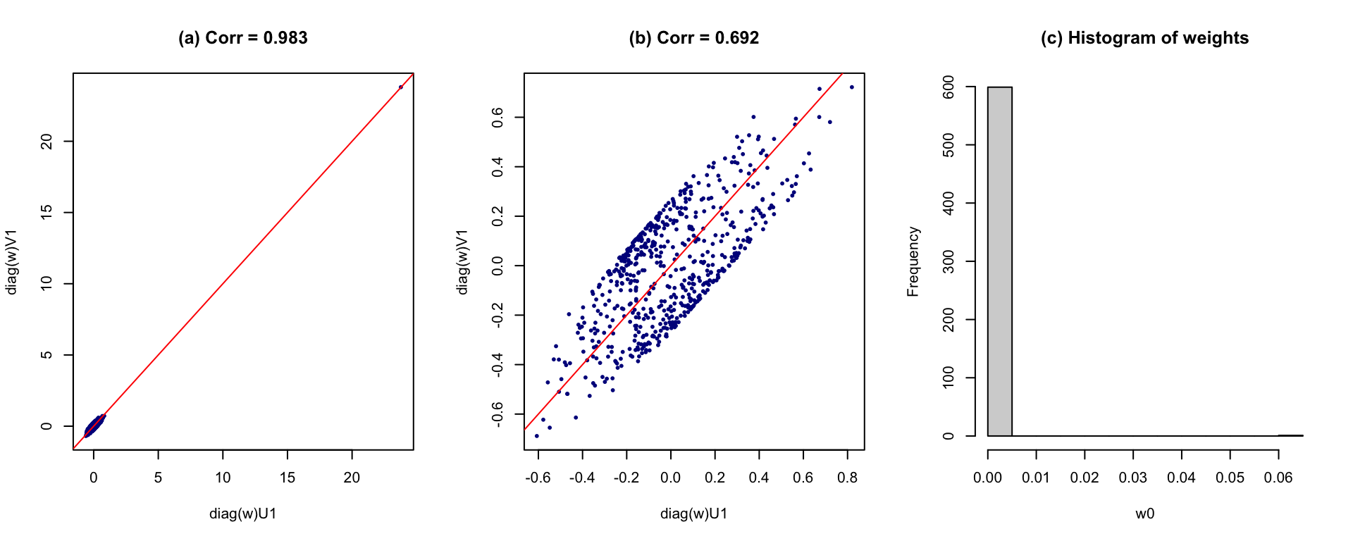
Figure 2: Results after weighting on subjects. (a) All data; (b) removing the influencial point; (c) histogram of weights

One way to handle this issue is to adopt a different penalty term that are more sensitive to the influential point. One potential proposal could be $max_{u, v, w} corr (diag (w) X u, diag (w) Y v) - λ | | w | |_{\infty}$ which penalize on the maximal $w$ . The results are listed below. From panel (b) in Figure 3, we see a clear difference in weights of subjects, which might imply a pattern of subgroups.

## [1] "Objective function value: 0.8839 (Loop1)"
## [1] "Objective function value: 0.8796 (Loop2)"
## [1] "Objective function value: 0.8888 (Loop3)"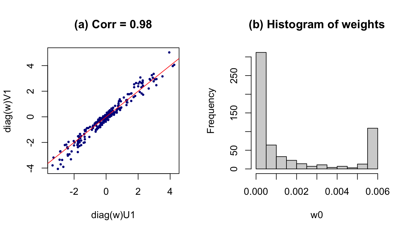

Figure 3: Results after weighting on subjects. (a) All data; (b) Histogram of weights