1 A General Framework
2 Multi-arm Treatment Effect Estimation
- 2.1 Q-learning
  - 2.1.1 S-learner
  - 2.1.2 T-learner
- 2.2 A-learning
3 Optimal Treatment Recommendation
- 3.1 Optimal Treatment Regimes
  - 3.1.1 Optimal Dynamic Treatment Regimes (DTR)
References

A corresponding Meta-learner R-package can be found on Github by the same author.

1 A General Framework

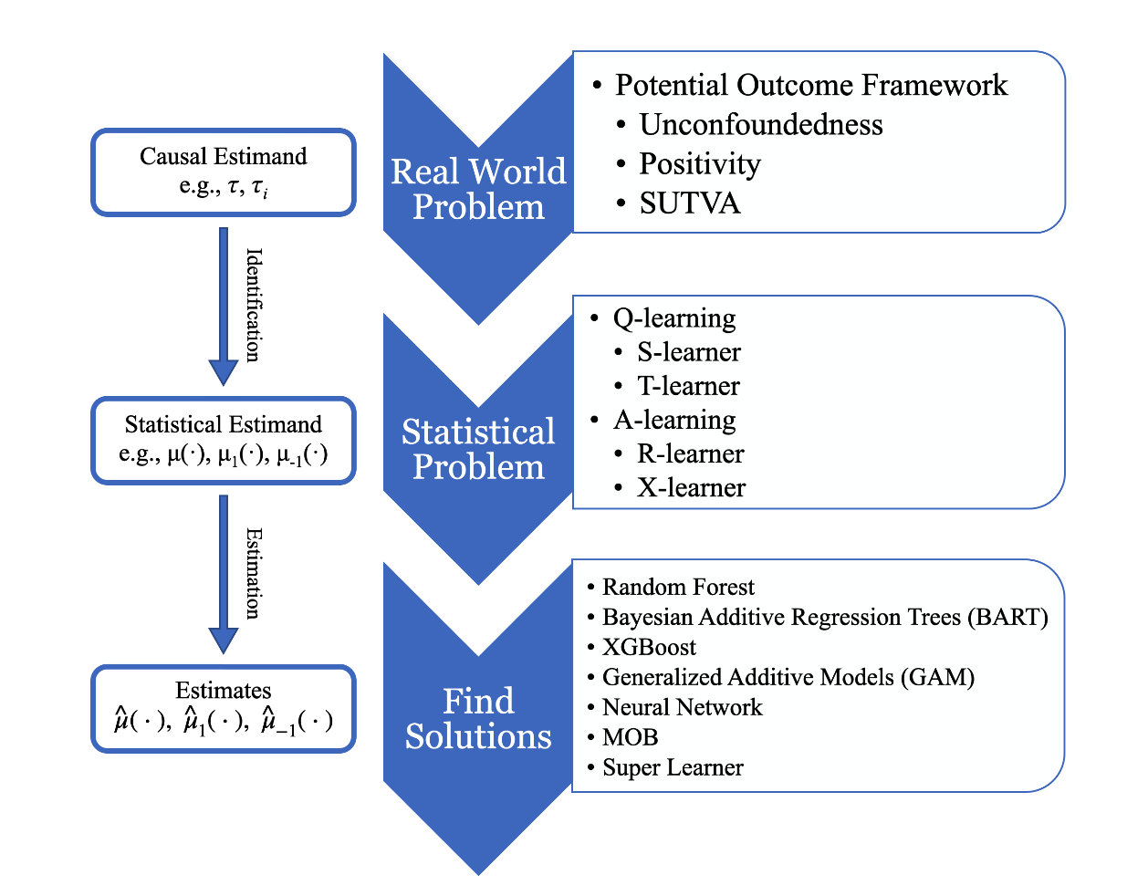
Meta-learners are a simple way to leverage off-the-shelf predictive machine learning methods to estimate conditional average treatment effect (CATE), heterogeneous treatment effect (HTE), and individual treatment effect (ITE). A very general process of doing causal inference is provided in the following flowchart, where there are three main parts:

Understand the real world question: what is the desired causal estimand/quantity. By potential outcome framework along with several assumptions, the causality could be inferred from the observed data, even without the randomized experiments, which is the gold standard for causal inference.
In step 2, the original real world problem is transformed to a solvable statistical problem with the assumption made in the first step. Usually, there could be different ways to form the statistical problem with pros and cons. As introduced in Review of Causal Inference: An Overview, there are T-learner and S-learner following the Q-learning approach as well as A-learning-based methods such as R-learner and X-learner.
After step 2, the statistical problem is built up, so in step 3, the main focus is how to solve them. If viewing in machine learning perspective, step 2 actually yields a problem specific loss function no matter following Q-learning or A-learning approach. The strength of meta-learners is they do not have strong requirements or limitations on the structure of loss function so that any off-the-shelf base learners can be readily fill in to solve. Such as Random Forests (RF) (Breiman 2001), Bayesian Additive Regression Trees (BART) (Chipman et al. 2010), XGBoost (Chen and Guestrin 2016), Generalized Additive Model (GAM) (Hastie and Tibshirani 1986), Neural Network (NN) (Hopfield 1982), Model-Based recursive partitioning (MOB) (Seibold et al. 2016; Zeileis et al. 2008), and Super Learner (SL) (Van der Laan et al. 2007).

2 Multi-arm Treatment Effect Estimation

Most causal inference literature study the treatment effect estimation under two-arm setting; for details, please refer to my another post Review of Causal Inference: An Overview. In this work, we work under a more generalized setting that there could be multiple arms.

2.1 Q-learning

Q-learning gets its name because its objective function plays a role similar to that of the Q or reward function in reinforcement learning (Murphy 2003; Murphy 2005a; Sutton and Barto 2018) and is widely used in estimating optimal dynamic treatment regime (Murphy et al. 2001; Murphy 2003, 2005b; Qian and Murphy 2011; Robins 2004; Schulte et al. 2014). The basic idea of Q-learning is to estimate the conditional response surfaces $E [Y ∣ X, T]$ , where $Y$ is the continuous outcome, $X$ represents the baseline covariates, and $T$ is the treatment assignment. In two-arm scenario, usually $T \in {0, 1}$ , and if there are $K$ treatment options, $T \in {1, 2, . . ., K}$ . After obtaining the Q-functions, the treatment effects can be estimated by contrasting these Q-functions. Q-learning is also known as g-computation (Robins 1986), or the parametric g-formula (Hernán and Robins 2010) in the literature. Though it is an indirect method in terms of treatment effect estimation, the performance is very competitive in practice, especially when the unconfoundedness assumption holds (Chatton et al. 2020).

In particular, to estimate Q-function, we here consider two approaches, one is Single or S-learner and the other is Two or T-learner method–following the nomenclature in Künzel et al. (2019). Both methods can be easily implemented in either two-arm or multi-arm settings. Notably, here S-, T-, and the following X-, and R-learner, they are merely general frameworks for treatment effect estimation, and in practice, people need to pick proper base learner for their scientific problem, such as Random Forest, BART, XGBoost, and etc., to implement these learners.

2.1.1 S-learner

For S-learner, we estimate a joint function $\hat{μ} (X, T) = E [Y ∣ X, T]$ with $T \in {1, 2, . . ., K}$ then the HTE between treatment $i$ and $j$ , $i \neq j$ , can be found by ${\hat{τ}}_{i}^{(j)} (X) = \hat{μ} (X, j) - \hat{μ} (X, i) .$ The whole data is used to estimate function $μ ()$ but since treatment $T$ is considered as one of the covariates, it can be neglected or underweighted if $X$ has high dimension. In practice, people usually reconstruct the design matrix by $[X, T, T \cdot X]$ , i.e., including the interaction terms to highlight the effects of $T$ (Lipkovich et al. 2011, 2017; Tian et al. 2014).

2.1.2 T-learner

T-learner, on the other hand, estimate $E [Y ∣ X, T]$ which only use part of the observed data. For example, when there are $K$ treatments, a total of $K$ functions need to by estimated, i.e., $μ_{k} (X) = E [Y ∣ X, T = k]$ for $k = 1, . . ., K$ . Then, the HTE can be calculated by ${\hat{τ}}_{i}^{(j)} (X) = {\hat{μ}}_{j} (X) - {\hat{μ}}_{i} (X)$ But it can lose the data efficiency due to the fact that each model is estimated separately.

2.2 A-learning

The main difference of advantage-learning or A-learning comparing to Q-learning, is to estimate targeted treatment effect $τ (x)$ directly. Unlike Q-learning is straightforward in understanding and implementation, A-learning need to formulate the unobserved treatment effect (e.g., ITE) first and then do the estimation. The X-learner and R-learner are considered under this framework. Both approaches are initially proposed for two treatments scenario, so here we extend them for multi-arm settings.

2.2.1 X-learner

X-learner (Künzel et al. 2019) enjoys the simplicity of T-learner but fixes its data efficiency issue by targeting on the treatment effects rather than the response surfaces. The main procedure for two-treatment setting is (denote two treatments as $1$ and $- 1$ )

Step 1: Estimate ${\hat{μ}}_{1} (\cdot)$ and ${\hat{μ}}_{- 1} (\cdot)$ just like T-learner
Step 2a: Impute ITEs for subjects in $T = 1$ arm by ${\tilde{τ}}_{1, i} = Y_{i} - {\hat{μ}}_{- 1} (x_{i})$ (recall that $τ_{i} = Y_{i}^{(1)} - Y_{i}^{(- 1)}$ ) and ITEs for subjects in $T = - 1$ arm by ${\tilde{τ}}_{- 1, i} = {\hat{μ}}_{1} (x_{i}) - Y_{i}$
Step 2b: Fit one model ${\hat{τ}}_{1} (\cdot)$ to predict ${\tilde{τ}}_{1, i}$ using data in $T = 1$ arm, i.e., ${(x_{i}, Y_{i})}_{i : T_{i} = 1}$ ; and fit another model ${\hat{τ}}_{- 1} (\cdot)$ to predict ${\tilde{τ}}_{- 1, i}$ using data in $T = - 1$ arm, i.e., ${(x_{i}, Y_{i})}_{i : T_{i} = - 1}$
Step 3: Combine ${\hat{τ}}_{1} (\cdot)$ and ${\hat{τ}}_{- 1} (\cdot)$ to achieve the final treatment effect model $\hat{τ} (x) = g (x) τ_{- 1} (x) + (1 - g (x)) τ_{1} (x)$ , where $g (\cdot)$ is some weighting function, e.g., propensity score.

For multi-arm setting, we can extend it with the same gist

Step 1: Estimate ${\hat{μ}}_{k} (\cdot), k = 1, . . ., K$ just like T-learner
Step 2a: For any pairwise HTE, for example, $τ_{i}^{(j)} (X) = E [Y ∣ T = j, X] - E [Y ∣ T = i, X]$ , we can have two sets of imputations: ${{\tilde{τ}}_{i, s}^{(j)} : Y_{s} - {\hat{μ}}_{i} (X_{s})}_{s : T_{s} = j}$ and ${{\tilde{τ}}_{i, s}^{(j)} : {\hat{μ}}_{j} (X_{s}) - Y_{s}}_{s : T_{s} = i}$
Step 2b: Fit one model for each imputed HTE which yields two models, denote ${\hat{τ}}_{i, i}^{(j)} (\cdot)$ which is estimated from subset ${{\tilde{τ}}_{i, s}^{(j)}}_{s : T_{s} = i}$ and ${\hat{τ}}_{i, j}^{(j)} (\cdot)$ which is estimated from ${{\tilde{τ}}_{i, s}^{(j)}}_{s : T_{s} = j}$
Step 3: Combine ${\hat{τ}}_{i, i}^{(j)} (\cdot)$ and ${\hat{τ}}_{i, j}^{(j)} (\cdot)$ to obtain final estimate ${\hat{τ}}_{i}^{(j)} (\cdot) = g (\cdot) {\hat{τ}}_{i, i}^{(j)} (\cdot) + (1 - g (\cdot)) {\hat{τ}}_{i, j}^{(j)} (\cdot)$ , where $g (\cdot)$ can be related with estimated propensity scores $g (\cdot) = {\hat{π}}^{(j)} / ({\hat{π}}^{(i)} + {\hat{π}}^{(j)})$

The underlying idea of X-learner is easy to understand: it tries to impute the missing outcomes first via the estimated Q-functions from the X-learner. After obtaining the pseudo ITE $\tilde{τ}$ of each subjects, it can then modeling on the treatment effect directly, which make it belong to A-learning framework. The authors justified that comparing to T-learner, X-learner is more robust when treatment allocation is unbalanced, i.e., one treatment is outnumbered the other in the observational dataset (Künzel et al. 2019). One potential issue of X-learner is, it is constructed based on squared loss function, which means it only applies for continuous outcomes but not for other outcome types, so far.

2.2.2 R-learner

R-learner (Nie and Wager 2020) adopts the Robinson’s decomposition (Robinson 1988) to connect the HTE with the observed quantities, ${Y, X, T}$ , $\begin{matrix} (2.1) & E [Y ∣ X, T] = m (X) + (1 [T = 1] - π (X)) τ (X) \end{matrix}$ where $m (X) = E [Y ∣ X]$ and $π (X) := Pr (T = 1 ∣ X)$ is the propensity score given covariates $X$ . The essence of Robinson’s decomposition is it separates out the target treatment effect $τ ()$ explicitly, which allows the further learning about $τ ()$ directly. That is the reason R-learner also belongs to A-learning framework.

Equation (2.1) is a two-arm version of R-learner. Following (citation), the loss function of R-learner in multi-arm setting is $\begin{matrix} (2.2) & \arg min_{τ_{i}} E [{(Y - m (X) - \sum_{k \neq i} (1 [T = k] - π^{(k)} (X)) τ_{i}^{(k)} (X))}^{2}] \end{matrix}$ where we denote the reference-specific treatment effects as $τ_{i} = (τ_{i}^{(1)}, . . ., τ_{i}^{(k - 1)}, τ_{i}^{(k + 1)}, . . ., τ_{i}^{(K)})$ . In practice, we can estimate $\hat{m} ()$ and $\hat{π} ()$ in the first stage and plug in to obtain ${\hat{τ}}_{i}$ once reference group $i$ is picked. However, with different reference group $i$ selection, loss functions (2.2) are different so that we can have $K$ sets of estimates: ${\hat{τ}}_{1}, . . ., {\hat{τ}}_{K}$ , which can lead to inconsistent HTE estimation as well as the optimal treatment recommendations. In practice, this could raise some concern and limitations (Zhou et al.).

Similar to X-learner, R-learner is also designed for continuous outcomes due to the limitation of Robinson’s decomposition.

2.2.3 Reference-free R-learner

To deal with the inconsistency recommendation problem in R-learner, the author propose a new method called reference-free R-learner (Zhou et al.) which allows to estimate treatment effect and recommend optimal treatment without specifying a particular reference group. So inconsistency issue is no longer a concern.

The essence of reference-free learner is to reformat the HTE $τ^{(k)}$ as a contrast between potential outcome $Y^{(k)}$ and outcome $Y$ , defined as $\begin{matrix} (2.3) & τ^{(k)} (X) = E [Y^{(k)} - Y ∣ X] = E [Y ∣ T = k, X] - E [Y ∣ X], for k = 1, . . ., K . \end{matrix}$ This definition allows us to sidestep the requirement of a reference treatment. Under this definition, traditional two-arm pairwise comparisons among different treatments can still be made as $τ_{j}^{(k)} (X) = E [Y^{(k)} - Y^{(j)} ∣ X] \equiv τ^{(k)} (X) - τ^{(j)} (X) .$

Then, following Robinson’s idea of decomposition (Robinson 1988), it yields $\begin{aligned} E [Y ∣ T, X] & = E [\sum_{k = 1}^{K} 1 [T = k] Y^{(k)} | T, X] = \sum_{k = 1}^{K} 1 [T = k] (E (Y ∣ X) + τ^{(k)} (X)) \\ (2.4) & = m (X) + \sum_{k = 1}^{K} 1 [T = k] τ^{(k)} (X), k = 1, . . ., K . \end{aligned}$ That is, we now have a different way to separate HTE out of the observations as described in (2.4) which no longer relies on the reference group as R-learner did. For implementation, we considering finding $\hat{τ} (\cdot)$ from the following objective function $\begin{aligned} \hat{τ} (\cdot) = \arg min_{τ} & \frac{1}{n} \sum_{i = 1}^{n} {(Y_{i} - \hat{m} (X_{i}) - \sum_{k = 1}^{K} 1 [T_{i} = k] τ^{(k)} (X_{i}))}^{2} \\ s.t. & \sum_{k = 1}^{K} τ^{(k)} (X_{i}) {\hat{π}}^{(k)} (X_{i}) = 0, i = 1, 2, . . ., n . \end{aligned}$ However, such optimization problem involves subjects dependent constraints, i.e., there will be $n$ constraints if there are $n$ subjects/datalines. Putting these constraints into objective function as penalty clearly won’t yield exact solution especially when $n$ is large. In their paper, the author proposed a nice and easy solution by projecting the original problem onto a simplex-spanned space where the constraints are satisfied implicitly. For more technical details, please refer to Zhou et al.

2.2.4 de-Centralized-Learner

(Author proposed learner which structured for causal inference analysis. Easy to implement and has superior performance comparing to the other meta-learners. For details, please wait for the publication.)

3 Optimal Treatment Recommendation

For S- and T-learner, the optimal treatment given covariate $x$ can be directly derived from $T^{opt} = \arg max_{k} \hat{μ} (x, k)$ for S-learner and $T^{opt} = \arg max_{k} {\hat{μ}}_{k} (x)$ for T-learner, suppose the larger outcome the better.

Since X-learner returns all possible pairwise treatment comparisons, ${\hat{τ}}_{i}^{(j)} (X)$ for $i = 1, . . ., K$ , $j = 1, . . ., K$ , and $i \neq j$ , the optimal treatment should be selected with a carefully designed decision rule to handle situations like ${\hat{τ}}_{1}^{(2)} (X) > 0$ , ${\hat{τ}}_{2}^{(3)} (X) > 0$ , and ${\hat{τ}}_{3}^{(1)} (X) > 0$ (given $K = 3$ ). Here we do not discuss how to choose a proper decision rule for pairwise comparison because it is out of the scope.

For R-learner, given a set of estimated HTE, ${\hat{τ}}_{j}$ , the optimal treatment can be determined by $T^{opt} = {\begin{cases} j & if {\hat{τ}}_{j}^{(k)} (X) < 0 for k \neq j, \\ \arg max_{k} {{\hat{τ}}_{j}^{(k)} (X), k = 1, 2, . . ., K} & else. \end{cases}$ But as aforementioned, the choice of $j$ leads to different set of ${\hat{τ}}_{j}$ , and correspondingly, different optimal recommendation $T^{opt}$ . That is, the selection of treatment group can cause various optimal recommendations.

3.1 Optimal Treatment Regimes

Meta-learner-based approaches find optimal treatment regimes by first estimate the treatment effect and then determine the optimal treatment accordingly. Another branch of methods, however, bypass the needs of estimating treatment effect but directly find the optimal treatment regimes. The reshape the problem as a weighted classification problem and then, many classification tools like SVM and trees can be used to solve the problem (Qian and Murphy 2011; Xu et al. 2015; Zhao et al. 2012; Zhu et al. 2017). Please check the basic idea of these approaches in my another post.

3.1.1 Optimal Dynamic Treatment Regimes (DTR)

In this whole work, we focus on the study with only one time of intervention. However, in practice, multiple-stage interventions may occur and how to determine the optimal sequence of treatments is therefore a natural question. It needs to highlight that subjects cannot be simply treated by the optimal treatment at each stage because the treatment effect may interact with each other and such greedy-algorithm-like idea cannot justify the carry-over effect. Q-learning and A-learning along with the dynamic programming is proposed to learn the optimal DTR from the Sequential, Multiple, Assignment Randomized Trials (SMART) (Lavori and Dawson 2000; Murphy 2005b; Nahum-Shani et al. 2012). If with proper causal assumptions, we can also learn the DTR from the observational studies as well with meta-learners. Since this is a big topic, we illustrate it in my another post in details along with some example codes for better demonstration.

References

Breiman, L. (2001), “Random forests,” Machine learning, Springer, 45, 5–32.

Chatton, A., Le Borgne, F., Leyrat, C., Gillaizeau, F., Rousseau, C., Barbin, L., Laplaud, D., Léger, M., Giraudeau, B., and Foucher, Y. (2020), “G-computation, propensity score-based methods, and targeted maximum likelihood estimator for causal inference with different covariates sets: A comparative simulation study,” Scientific reports, Nature Publishing Group, 10, 1–13.

Chen, T., and Guestrin, C. (2016), “XGBoost: A scalable tree boosting system,” in Proceedings of the 22nd ACM SIGKDD international conference on knowledge discovery and data mining, KDD ’16, New York, NY, USA: Association for Computing Machinery, pp. 785–794. https://doi.org/10.1145/2939672.2939785.

Chipman, H. A., George, E. I., McCulloch, R. E., and others (2010), “BART: Bayesian additive regression trees,” The Annals of Applied Statistics, Institute of Mathematical Statistics, 4, 266–298.

Hastie, T., and Tibshirani, R. (1986), “Generalized additive models,” Statistical Science, JSTOR, 297–310.

Hernán, M. A., and Robins, J. M. (2010), “Causal inference,” CRC Boca Raton, FL;

Hopfield, J. J. (1982), “Neural networks and physical systems with emergent collective computational abilities,” Proceedings of the national academy of sciences, National Acad Sciences, 79, 2554–2558.

Künzel, S. R., Sekhon, J. S., Bickel, P. J., and Yu, B. (2019), “Metalearners for estimating heterogeneous treatment effects using machine learning,” Proceedings of the National Academy of Sciences, National Acad Sciences, 116, 4156–4165.

Lavori, P. W., and Dawson, R. (2000), “A design for testing clinical strategies: Biased adaptive within-subject randomization,” Journal of the Royal Statistical Society: Series A (Statistics in Society), Wiley Online Library, 163, 29–38.

Lipkovich, I., Dmitrienko, A., and B D’Agostino Sr, R. (2017), “Tutorial in biostatistics: Data-driven subgroup identification and analysis in clinical trials,” Statistics in medicine, Wiley Online Library, 36, 136–196.

Lipkovich, I., Dmitrienko, A., Denne, J., and Enas, G. (2011), “Subgroup identification based on differential effect search—a recursive partitioning method for establishing response to treatment in patient subpopulations,” Statistics in medicine, Wiley Online Library, 30, 2601–2621.

Murphy, S. A. (2003), “Optimal dynamic treatment regimes,” Journal of the Royal Statistical Society: Series B (Statistical Methodology), Wiley Online Library, 65, 331–355.

Murphy, S. A. (2005a), “A generalization error for q-learning,” Journal of Machine Learning Research, 6, 1073–1097.

Murphy, S. A. (2005b), “An experimental design for the development of adaptive treatment strategies,” Statistics in medicine, Wiley Online Library, 24, 1455–1481.

Murphy, S. A., Laan, M. J. van der, Robins, J. M., and Group, C. P. P. R. (2001), “Marginal mean models for dynamic regimes,” Journal of the American Statistical Association, Taylor & Francis, 96, 1410–1423.

Nahum-Shani, I., Qian, M., Almirall, D., Pelham, W. E., Gnagy, B., Fabiano, G. A., Waxmonsky, J. G., Yu, J., and Murphy, S. A. (2012), “Experimental design and primary data analysis methods for comparing adaptive interventions.” Psychological methods, American Psychological Association, 17, 457.

Nie, X., and Wager, S. (2020), “Quasi-oracle estimation of heterogeneous treatment effects,” Biometrika, 108, 299–319. https://doi.org/10.1093/biomet/asaa076.

Qian, M., and Murphy, S. A. (2011), “Performance guarantees for individualized treatment rules,” Annals of statistics, NIH Public Access, 39, 1180.

Robins, J. (1986), “A new approach to causal inference in mortality studies with a sustained exposure period—application to control of the healthy worker survivor effect,” Mathematical modelling, Elsevier, 7, 1393–1512.

Robins, J. M. (2004), “Optimal structural nested models for optimal sequential decisions,” in Proceedings of the second seattle symposium in biostatistics, Springer, pp. 189–326.

Robinson, P. M. (1988), “Root-n-consistent semiparametric regression,” Econometrica, [Wiley, Econometric Society], 56, 931–954.

Schulte, P. J., Tsiatis, A. A., Laber, E. B., and Davidian, M. (2014), “Q-and a-learning methods for estimating optimal dynamic treatment regimes,” Statistical science: a review journal of the Institute of Mathematical Statistics, NIH Public Access, 29, 640.

Seibold, H., Zeileis, A., and Hothorn, T. (2016), “Model-based recursive partitioning for subgroup analyses,” The international journal of biostatistics, De Gruyter, 12, 45–63.

Sutton, R. S., and Barto, A. G. (2018), Reinforcement learning: An introduction, MIT press.

Tian, L., Alizadeh, A. A., Gentles, A. J., and Tibshirani, R. (2014), “A simple method for estimating interactions between a treatment and a large number of covariates,” Journal of the American Statistical Association, Taylor & Francis, 109, 1517–1532.

Van der Laan, M. J., Polley, E. C., and Hubbard, A. E. (2007), “Super learner,” Statistical applications in genetics and molecular biology, De Gruyter, 6.

Xu, Y., Yu, M., Zhao, Y.-Q., Li, Q., Wang, S., and Shao, J. (2015), “Regularized outcome weighted subgroup identification for differential treatment effects,” Biometrics, Wiley Online Library, 71, 645–653.

Zeileis, A., Hothorn, T., and Hornik, K. (2008), “Model-based recursive partitioning,” Journal of Computational and Graphical Statistics, Taylor & Francis, 17, 492–514.

Zhao, Y., Zeng, D., Rush, A. J., and Kosorok, M. R. (2012), “Estimating individualized treatment rules using outcome weighted learning,” Journal of the American Statistical Association, Taylor & Francis, 107, 1106–1118.

Zhou, J., Zhang, Y., and Tu, W.“A reference-free r-learner for treatment recommendation,” Statistical Methods in Medical Research, 0, 09622802221144326. https://doi.org/10.1177/09622802221144326.

Zhu, R., Zhao, Y.-Q., Chen, G., Ma, S., and Zhao, H. (2017), “Greedy outcome weighted tree learning of optimal personalized treatment rules,” Biometrics, Wiley Online Library, 73, 391–400.