An under-developing metaDTR R-package can be found on Github by the same author.

Introduction

“Dynamic treatment regimes (DTRs), also called treatment policies, adaptive interventions or adaptive treatment strategies, were created to inform the development of health-related interventions composed of sequences of individualized treatment decisions. These regimes formalize sequential individualized treatment decisions via a sequence of decision rules that map dynamically evolving patient information to a recommended treatment. An optimal DTR optimizes the expectation of a desired cumulative outcome over a population of interest. An estimated optimal DTR has the potential to:

improve patient outcomes through adaptive personalized treatment;
reduce treatment burden and resource demands by recommending treatment only if, when, and to whom it is needed; and
generate new scientific hypotheses about heterogeneous treatment effects over time both across and within patients.”(Laber et al. 2014)

We consider the development of DTRs using data from Sequential, Multiple, Assignment Randomized Trials (SMART) (Lavori and Dawson 2000; Murphy 2005a; Nahum-Shani et al. 2012). See Figure 1 for a concrete example of a hypothetical SMART design for addiction management that is introduced in Chakraborty and Murphy (2014). “In this trial, each participant is randomly assigned to one of two possible initial treatments: cognitive behavioral therapy (CBT) or naltrexone (NTX). A participant is classified as a non-responder or responder to the initial treatment according to whether s/he does or does not experience more than two heavy drinking days during the next two months. A non-responder to NTX is re-randomized to one of the two subsequent treatment options: either a switch to CBT, or an augmentation of NTX with CBT (CBT+NTX). Similarly, a non-responder to CBT is re-randomized to either a switch to NTX, or an augmentation (CBT+NTX). Responders to the initial treatment receive telephone monitoring (TM) for an additional period of six months. One goal of the study might be to construct a DTR leading to a maximal mean number of non-heavy drinking days over 12 months.” (Chakraborty and Murphy 2014)

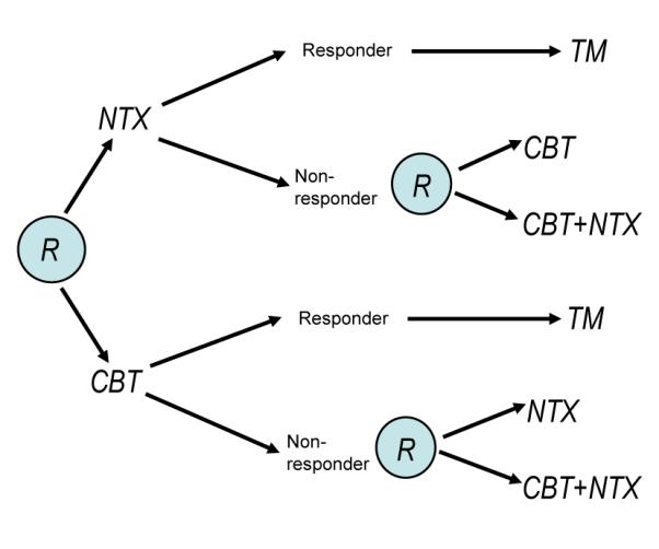
Hypothetical SMART design schematic for the addiction management example (an 'R' within a circle denotes randomization at a critical decision point)

Figure 1: Hypothetical SMART design schematic for the addiction management example (an ‘R’ within a circle denotes randomization at a critical decision point)

DTRs offer a framework for operationalizing the adaptive decision making in clinical practice and thereby potentially improving it. They can be conceptualized as decision support systems for the clinicians-one of the key elements of the Chronic Care Model (Wagner et al. 2001).

Before moving to technical details of optimizing DTR, we here discuss a little bit about why not combining best treatment at each stage that are obtained from separate randomized trials. This way does not necessarily give the optimal DTR, due to:

Delayed Therapeutic Effect

Treatment I may not appear best initially but may have enhanced long term effectiveness when followed by a particular “maintenance” treatment (Positive Synergies)
Treatment I may produce a higher proportion of responders but also result in side effects that reduce the variety of subsequent treatments for those that do not respond, Or the burden imposed by treatment I may be sufficiently high so that non-responders are less likely to adhere to subsequent treatments (Negative Synergies)

Diagnostic Effect or Prescriptive Effect

Treatment I may produce a lesser proportion of responders that treatment II, but treatment I may elicit symptoms that allow the investigator to better match subsequent treatment to the patient and thus achieve improved primary outcome to the sequence of treatments as compared to initial treatment II

Cohort Effect or Selection Effect

Subjects who enroll in, or who remain in or who are adherent in the trial of the initial treatments may be quite different from the subjects in SMART

In this work, we will introduce the overall structure of finding the optimal DTRs using backward induction. Moreover, we incorporate the idea of meta-learners, which are frequently used in causal inference for optimal treatment recommendation and/or heterogeneous treatment effect estimation, to facilitate the estimation of DTRs. We also evaluate the performance of the proposed meta-learner methods with the existing state-of-art methods using the same simulation setting.

Method

Notation and Problem Setup

Consider a multistage decision problem where decisions are made at $T$ . Here we use capital letters to represent random variables and lower case for observations. For $t = 1, . . ., T$ , let $A_{t}$ denote the treatment assigned at the $t^{t h}$ stage, and $X_{t}$ be the observations after treatment assignment $A_{t - 1}$ but prior to $A_{t}$ . In particular, $X_{1}$ stands for the baseline covariates, while $X_{t}, t > 1$ are merely a realization of one “potential” set of covariates corresponding to the history treatment sequence $a_{1}, . . ., a_{t - 1}$ . In other words, the covariates observed at later stage might be impacted by the past treatment assignments. Notably, $A_{j}$ might be multi-category or even continuous, but to ease illustration, we mainly focus on binary treatment scenario, i.e., $A_{t} \in {0, 1}, t = 1, . . ., T$ in this section, and will discuss the cases with $K$ treatment options $A_{t} \in {1, . . ., K}$ in later sections. See Figure 2 for a better understanding of the notation in a two-stage study design.

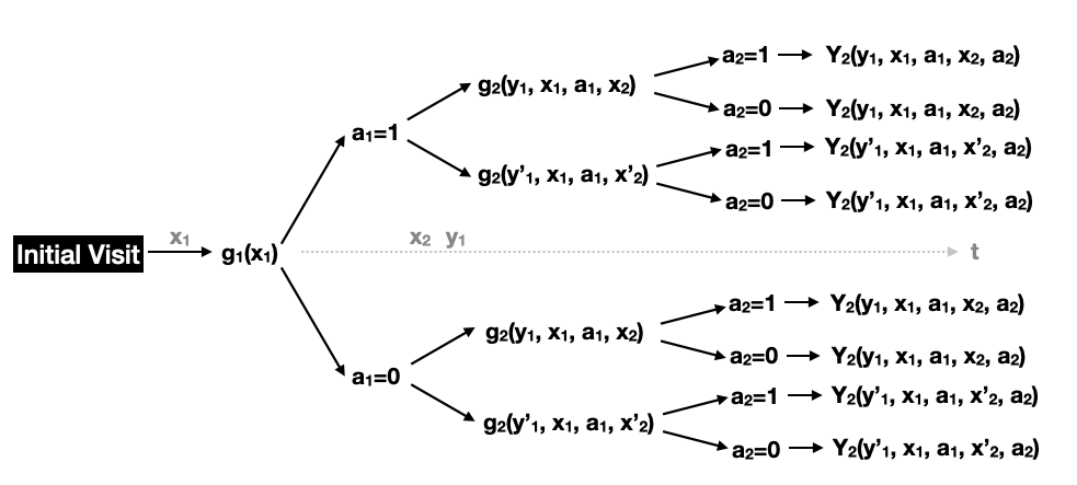
Figure 2: A two-stage study design

Following $t^{t h}$ treatment, there will be an observed outcome, or so-called “reward” in the reinforcement learning researches, denoted as $Y_{t}$ , where the larger the better in current setting. Usually, the outcome depends on the whole history information, i.e., all the covariates observed before $t^{t h}$ stage, $X_{1}, . . ., X_{t}$ ; all the treatment assignments $A_{1}, . . ., A_{t}$ ; and all past outcomes $Y_{1}, . . . Y_{t - 1}$ . For simplicity in notation, we use $H_{t} = (X_{1}, A_{1}, Y_{1}, . . ., A_{t - 1}, Y_{t - 1}, X_{t})$ to represent the history information available at stage $t$ .

The goal of DTR is to maximize the total rewards/outcomes: $Y^{*} = \sum_{t = 1}^{T} w_{t} Y_{t},$ where $w_{t}$ represent the pre-defined weighting factors for outcomes at each stage. Weighting helps to flexibly customize the goal for a specific question. In trial design, usually people adopt equal weights, but in finance, for example, it’s quite natural to choose $w_{t} = {(\frac{1}{1 + r_{f}})}^{t}, t = 1, . . ., T$ to maximize the present value by discounting the future cash flows. $r_{f}$ can be the risk-free rate like 10 Year Treasure Rate.

A dynamic treatment regime (DTR) is an ordered set of deterministic decision rules, denoted as $g = (g_{1}, . . ., g_{T})$ , where $g_{t}$ is a map from the space of $H_{t}$ to the available assignment space $A_{t}$ , i.e., $g_{t} : H_{t} ⟼ A_{t}$ . Let $Y^{*} (g)$ be the outcome given treatments follows the regime $g$ , and then the optimal treatment regime $g^{opt} = (g_{1}^{opt}, . . ., g_{T}^{opt})$ should satisfy $\begin{matrix} (1) & E [Y^{*} (g^{opt})] \geq E [Y^{*} (g)], g \in G \end{matrix}$ where $G$ is the class of all feasible regimes.

To find solution for $g$ satisfies equation (1), the most common way is called Q-learning, which is an indirectly method. On the other hand, people could also use directly method, namely, A-learning to seek solution. In later subsections, we will introduce the basic idea of these two methods.

Q-learning

The optimal regime may be determined via dynamic programming, also referred to as backward induction (Bellman 1966; Murphy et al. 2001; Murphy 2003). Define Q-functions, with “Q” for “quality”, as $\begin{aligned} Q_{T} (h_{T}, a_{T}) & = E [Y_{T} ∣ H_{T} = h_{T}, A_{T} = a_{T}], \\ Q_{t} (h_{t}, a_{t}) & = E [Y_{t} + max_{a_{t + 1}} Q_{t + 1} (h_{t + 1}, a_{t + 1}) ∣ H_{t + 1} = h_{t + 1}, A_{t + 1} = a_{t + 1}] \end{aligned}$ for $t = T - 1, . . ., 1$ . The optimal treatment at each stage is then determined by $\begin{matrix} (2) & g_{t}^{opt} (h_{t}) = \arg max_{a_{t}} Q_{t} (h_{t}, a_{t}), t = 1, . . ., T . \end{matrix}$ Hence, the optimal DTR is $g^{opt} (h_{T}) = (g_{1}^{opt} (h_{1}), . . ., g_{T}^{opt} (h_{T}))$ . In practice, we need to first obtain $Q_{t} ()$ , then find $Q_{t - 1} ()$ , and repeat this procedure recursively until $t = 1$ . Since optimal DTR is totally dependent on the performance of estimated $Q_{1} (), . . ., Q_{T} ()$ , so this approach is named as “Q-learning”. In terms of how to obtain Q-functions, we introduce meta-learners to complete this task. Under the Q-learning umbrella, there are two main approaches, Single- or S-learner and Two- or T-learner.

S-learner

For simplicity, define value function $V_{t} (h_{t}) = max_{a_{t}} Q_{t} (h_{t}, a_{t})$ . Also, consider a target loss function $ℓ (q, \tilde{q})$ , which measures the “loss” between the observed quantity $q$ and estimated quantity $\tilde{q}$ . For continuous $q$ , for example, the loss function $ℓ ()$ could be mean squared error; for binary outcomes, it could be logit loss or simply Shannon entropy; or if $q$ is a distribution, then $ℓ ()$ can choose Kullback-Leibler divergence. In S-learner, we basically only need to use the base learner to minimize the following loss $\begin{matrix} (3) & {\hat{Q}}_{t} (h_{t}, a_{t}) = \arg min_{Q_{t}} ℓ (Y_{t + 1} + {\hat{V}}_{t + 1} (h_{t + 1}), Q_{t} (h_{t}, a_{t})) \end{matrix}$ where ${\hat{V}}_{t + 1} (\cdot)$ is obtained in the previous step; and then we can estimate ${\hat{V}}_{t} (h_{t}) = max_{a_{t}} {\hat{Q}}_{t} (h_{t}, a_{t})$ . By conducting this procedure recursively, we get $({\hat{Q}}_{1}, . . ., {\hat{Q}}_{T})$ and followed by ${\hat{g}}^{opt}$ . In practice, $Q ()$ is a known function of parameter $Θ$ and (3) is basically solving the following optimization problem ${\hat{Θ}}_{t} = \arg min_{Θ_{t}} ℓ (Y_{t + 1} + {\hat{V}}_{t + 1} (h_{t + 1}), Q_{t} (h_{t}, a_{t}; Θ_{t})) .$ For simplicity, we here try not to involve too much notation and therefore, we follow the structure of (3) instead hereafter.

T-learner

The only difference between S- and T-learner is, in S-learner, there is only one Q-function at each stage, while in T-learner, we estimate two Q-functions, one for $a_{t} = 1$ and the other for $a_{t} = 0$ . Specifically, we now have $\begin{aligned} {\hat{Q}}_{t, 1} (h_{t}) & = \arg min_{Q_{t, 1}} ℓ (Y_{t + 1} + {\hat{V}}_{t + 1} (h_{t + 1}), Q_{t, 1} (h_{t}) ∣ a_{t} = 1) \\ {\hat{Q}}_{t, 0} (h_{t}) & = \arg min_{Q_{t, 0}} ℓ (Y_{t + 1} + {\hat{V}}_{t + 1} (h_{t + 1}), Q_{t, 0} (h_{t}) ∣ a_{t} = 0) \end{aligned}$ and the corresponding estimation of value function is thus ${\hat{V}}_{t} (h_{t}) = max ({\hat{Q}}_{t, 1} (h_{t}), {\hat{Q}}_{t, 0} (h_{t})) .$ Notably, though $Q_{t} (h_{t}, a_{t})$ is similar to $Q_{t, a_{t}} (h_{t})$ conceptually, the former one is estimated using whole data, while the latter one only use part of data, i.e., either $a_{t} = 1$ subset or $a_{t} = 0$ . The rest are identical to S-learner.

To learn more about S- and T-learner, please refer to my another post.

Since Q-learning merely trains the outcomes rather than the treatment effect, so there might be error in determining the optimal treatment (Murphy 2005b). Also, this is the reason why it is known as indirect method. Therefore, another branch of methods are proposed under A-learning framework, which try to train directly on the treatment effect and obtain optimal treatment accordingly.

A-learning

A-learning is short for Advantage learning which is another main approach to seek optimal DTR (Blatt et al. 2004; Moodie et al. 2007; Murphy 2003; Robins 2004). We can define a contrast function in two arm scenario as $C_{t} (h_{t}) := E [Y_{t} ∣ H_{t} = h_{t}, A_{t} = 1] - E [Y_{t} ∣ H_{t} = h_{t}, A_{t} = 0]$ and the optimal treatment in terms of this contrast function can be written as $\begin{matrix} (4) & g_{t}^{opt} (h_{t}) = I (C_{t} (h_{t}) > 0), t = 1, . . ., T . \end{matrix}$ Remarkably, the contrast function is parallel to the treatment effect $τ ()$ in causal inference, which can be deemed as seeking optimal treatment regime in an one-stage design. In particular, if $A_{t}$ is a random assignment, or unconfoundedness assumption holds, that is, $(Y_{t}^{(1)}, Y_{t}^{(0)}) ⊥ A_{t} ∣ H_{t}$ then we have $C_{t} (h_{t}) = E [Y_{t}^{(1)} ∣ H_{t} = h_{t}] - E [Y_{t}^{(0)} ∣ H_{t} = h_{t}] = E [Y_{t}^{(1)} - Y_{t}^{(0)} ∣ H_{t} = h_{t}]$ which is the treatment effect. Here $Y_{t}^{(1)}$ and $Y_{t}^{(0)}$ are the potential outcome of receiving treatment 1 and 0 at $t^{t h}$ stage, respectively.

The value function for A-learning in terms of contrast function is $V_{t} (h_{t}) = Q_{t} (h_{t}, 0) + C_{t} (h_{t}) I (C_{t} (h_{t}) > 0)$ where Q-functions are still involved. To get rid of Q-functions, we can re-write it as $\begin{matrix} (5) & V_{t} (h_{t}) = V_{t + 1} (h_{t + 1}) + C_{t} (h_{t}) (I (C_{t} (h_{t}) > 0) - A_{t}) \end{matrix}$ and it is obvious that, in contrast to Q-learning, the optimal DTR of A-learning is fully determined by the performance of $C_{t} (), t = 1, . . ., T$ . In addition, we would like to provide some intuition of equation (5). If the predicted optimal treatments matches with the realized assignments, i.e., $g_{t}^{opt} (h_{t}) = A_{t}$ , then we do not need to make correction on next stage’s value function $V_{t + 1} (h_{t + 1})$ since it is already optimized; otherwise, we adjust it by the amount of $C_{t} (h_{t})$ . For instance, if the realized $A_{t} = 1$ but our estimation says it should be $0$ , then we correct the value function by the treatment effect difference, which is $- C_{t} (h_{t}) > 0$ . That will increase the future value functions and enlarge the overall rewards. This idea is inspired from Zhang and Zhang (2018).

Notably, if we estimate $C_{t} (h_{t})$ by ${\hat{C}}_{t} (h_{t}) = {\hat{Q}}_{t} (h_{t}, 1) - {\hat{Q}}_{t} (h_{t}, 0)$ , then optimal treatment found by equation (4) is identical to that of Q-learning (2). However, people can also bypass the estimation of Q-functions and directly find estimator for $C_{t} (h_{t})$ . So, ideally, A-learning is suppose to be more robust against model misspecification than Q-learning for consistent estimation of the optimal treatment regime (Schulte et al. 2014). There are a bunch of literature propose different ways to approach the contrast function or similar alternatives (Shi et al. 2018; Zhang et al. 2013; Zhang and Zhang 2018; Zhao et al. 2015). In the next subsection, we propose a novel method to estimate contrast function, which also follows the idea of meta-learner.

X-learner

X-learner is originally proposed for heterogeneous treatment effect estimation (Künzel et al. 2019). It fixes the data inefficiency in T-learner and also can outperform T-learner if unbalanced treatment allocation exists (Künzel et al. 2019). Here we extend X-learner for optimizing DTR, and the main procedure is summarized below:

Estimate ${\hat{Q}}_{t, 1} (h_{t})$ and ${\hat{Q}}_{t, 0} (h_{t})$ as described in T-learner
Impute missing potential “outcomes” by ${\hat{Q}}_{t, 1} (h_{t})$ and ${\hat{Q}}_{t, 0} (h_{t})$ . In particular, for subjects with $A_{t} = 1$ , their potential outcomes are predicted by ${\hat{Q}}_{t, 0} (h_{t}; a_{t} = 1)$ and then we can construct pseudo contrast values ${\tilde{C}}_{t} (h_{t}; a_{t} = 1) = Y_{t + 1} + {\hat{V}}_{t + 1} (h_{t + 1}) - {\hat{Q}}_{t, 0} (h_{t}; a_{t} = 1)$ for all subjects with assignments $A_{t} = 1$ . Next, we find the optimal contrast function by minimizing the loss function ${\hat{C}}_{t, 1} (h_{t}) = \arg min_{C_{t, 1}} ℓ ({\tilde{C}}_{t} (h_{t}; a_{t} = 1), C_{t, 1} (h_{t}))$ via some base learner. Similarly, we can find another contrast function ${\hat{C}}_{t, 0} (h_{t}) = \arg min_{C_{t, 0}} ℓ ({\tilde{C}}_{t} (h_{t}; a_{t} = 0), C_{t, 0} (h_{t}))$ for subjects with $A_{t} = 0$
Lastly, combine both contrast functions to achieve the final model. One recommended way is ${\hat{C}}_{t} (h_{t}) = {\hat{C}}_{t, 1} (h_{t}) (1 - {\hat{g}}_{t} (h_{t})) + {\hat{C}}_{t, 0} (h_{t}) {\hat{g}}_{t} (h_{t})$ where ${\hat{g}}_{t} ()$ can be the estimated propensity score values at $t^{t h}$ stage.

Simulation Studies

Case 1: Random assignment with two treatment options

In the first case, we follow the settings adopted in Zhao et al. (2015) and Zhang and Zhang (2018), which is 3-stage randomized study with only two treatment options. Treatment assignments at each stage $A_{1}$ , $A_{2}$ , and $A_{3}$ are randomly generated from a Bernoulli $(0.5)$ distribution. Baseline covariates as well as covariates observed at each stage is generated as follows: $\begin{aligned} X_{1, i} & \sim N (45, 15^{2}), i = 1, . . ., 10 \\ X_{2, i} & \sim N (1.5 X_{1, i}, 10^{2}), i = 1, . . ., 5 \\ X_{3, i} & \sim N (0.5 X_{2, i}, 10^{2}), i = 1, . . ., 5. \end{aligned}$ Outcomes or regrets are generated from $\begin{aligned} Y_{1} & = Y_{2} = 0, \\ Y_{3} & = 20 - | 0.6 X_{1, 1} - 40 | {A_{1} - I (X_{1, 1} > 30)}^{2} - | 0.8 X_{2, 1} - 60 | {A_{2} - I (X_{2, 1} > 40)}^{2} \\ - | 1.4 X_{3, 1} - 40 | {A_{3} - I (X_{3, 1} > 40)}^{2} + ε, where ε \sim N (0, σ^{2}) . \end{aligned}$ Here we take $σ = 1$ for fair comparison with results in existing literature. Since $Y_{1} = Y_{2} = 0$ , it means that we only care about the final outcome and intermediate returns are of no concerns. Also, from the formula of $Y_{3}$ , we can see that the expectation of optimal return should be 20, i.e., $E [Y^{*} (g^{opt})] = 20,$ where $\begin{aligned} g_{1}^{o p t} & = I (X_{1, 1} > 30) \\ g_{2}^{o p t} & = I (X_{2, 1} > 40) \\ g_{3}^{o p t} & = I (X_{3, 1} > 40) . \end{aligned}$ In this work, we adopt BART (Chipman et al. 1998, 2002, 2010) as base learner for implementation of S-, T-, and X-learner. BART is a powerful learning tool which enjoys the benefit of tree structure, boosting technique, and prior and likelihood, and it is also quite efficient in computation. We directly call the bart() function in R package dbarts (Dorie et al. 2022).

Example R code: S-learner

We first generate the simulated data as described in the previous section using the following code. The training set has 400 samples and the testing set has 1000 samples. A, X, and Y follow the notation in Method section that stand for the treatment assignments, covariates, and outcomes, respectively, and with a suffix tr means training data, te means testing data.

set.seed(54321)
n.sbj = 400; n.test = 1000; sigma = 1
n.stage = 3
nX1 = 10; nX2 <- nX3 <- 5
## Treatment Assignments A at each stage:
A.tr = matrix(rbinom(n.sbj*n.stage,1,0.5), ncol = n.stage)
## Observed covariates X before each stage:
X1.tr = matrix(rnorm(n.sbj*nX1, 45, 15), ncol = nX1)
X2.tr = matrix(rnorm(n.sbj*nX2, X1.tr[,1:nX2], 10), ncol = nX2)
X3.tr = matrix(rnorm(n.sbj*nX3, X2.tr[,1:nX3], 10), ncol = nX3)
## Outcome/Reward generator:
y.fun <- function(X1, X2, X3, A) {
  20 - abs(0.6*X1[,1])*abs(A[,1] - (X1[,1]>30)) -
  abs(0.8*X2[,1] - 60)*abs(A[,2] - (X2[,1]>40)) -
  abs(1.4*X3[,1] - 40)*abs(A[,3] - (X3[,1]>40))
}
Y.tr = y.fun(X1.tr, X2.tr, X3.tr, A.tr) + rnorm(n.sbj,0,sigma)
## test data:
X1.te = matrix(rnorm(n.test*nX1, 45, 15), ncol = nX1)
X2.te = matrix(rnorm(n.test*nX2, X1.tr[,1:nX2],10), ncol = nX2)
X3.te = matrix(rnorm(n.test*nX3, X2.tr[,1:nX3],10), ncol = nX3)

The code of applying S-learner on the simulated data to find the optimal DTR is given below. As there are 3 stages, we estimate the Q-functions for each stage separately in a backward order, i.e., we first find $Q_{3} ()$ , then $Q_{2} ()$ , and $Q_{1} ()$ at last. As long as we obtain these Q-functions, i.e., Q.S1, Q.S2, and Q.S3 in the following code, the optimal dynamic treatments for any given subjects are determined.

##+++++++++++++++++  Q-learning: S-learner style  +++++++++++++++++
### For stage 3 first:
S3.dat = cbind(X1.tr, X2.tr, X3.tr, A.tr[,-3], 1-A.tr[,3])
Q.S3 = bart(x.train = cbind(X1.tr, X2.tr, X3.tr, A.tr), y.train = Y.tr, 
            x.test = S3.dat,  # prediction for potential outcomes
            ntree = 200, verbose = FALSE, keeptrees = TRUE) 
V3.est = pmax(Q.S3$yhat.test.mean, Q.S3$yhat.train.mean) # find V_3

### Stage 2 then:
S2.dat = cbind(X1.tr, X2.tr, A.tr[,-c(2:3)], 1-A.tr[,2])
Q.S2 = bart(x.train = cbind(X1.tr, X2.tr, A.tr[, -3]), y.train = V3.est, 
            x.test = S2.dat,   # prediction for potential outcomes
            ntree = 200, verbose = FALSE, keeptrees = TRUE) 
V2.est = pmax(Q.S2$yhat.test.mean, Q.S2$yhat.train.mean) # find V_2

### Stage 1 last:
S1.dat = cbind(X1.tr, 1-A.tr[,1])
Q.S1 = bart(x.train = cbind(X1.tr, A.tr[, 1]), y.train = V2.est, 
            ntree = 200, verbose = FALSE, keeptrees = TRUE) 

### Prediction on Testing data
Y1.1 = colMeans(predict(Q.S1, newdata = cbind(X1.te, 1)))
Y1.0 = colMeans(predict(Q.S1, newdata = cbind(X1.te, 0)))
A1.te = ifelse(Y1.1>Y1.0, 1, 0)
Y2.1 = colMeans(predict(Q.S2, newdata = cbind(X1.te, X2.te, A1.te, 1)))
Y2.0 = colMeans(predict(Q.S2, newdata = cbind(X1.te, X2.te, A1.te, 0)))
A2.te = ifelse(Y2.1>Y2.0, 1, 0)
Y3.1 = colMeans(predict(Q.S3, newdata = cbind(X1.te, X2.te, X3.te, A1.te, A2.te, 1)))
Y3.0 = colMeans(predict(Q.S3, newdata = cbind(X1.te, X2.te, X3.te, A1.te, A2.te, 0)))
A3.te = ifelse(Y3.1>Y3.0, 1, 0)
A.opt.S = cbind(A1.te, A2.te, A3.te)

### Results
Y.origin = y.fun(X1.tr, X2.tr, X3.tr, A.tr)
Y.eva.S = y.fun(X1.te, X2.te, X3.te, A.opt.S)
mean(Y.origin)     # rewards from original assignments

## [1] -22.92242

mean(Y.eva.S)      # rewards from optimized assignments

## [1] 19.86825

mean(Y.eva.S==20)  # percentage that receive the best treatment seq.

## [1] 0.992

Focus on this simulated sample, we can see that in original study design, since subjects are randomized at each stage, the treatment effects are clearly not optimal, with mean outcome -22.92. However, after trained by S-learner, the average outcome following the optimized DTR can reach to 19.87 (the upper bound is 20), with 99.2% subjects receives the best treatment sequence for them.

Example R code: T-learner

With the same dataset, we now try T-learner. The code is shown below. Since we need to train two models for $A = 1$ and $A = 0$ separately, there are Q.S_.1 and Q.S_.0 at each stage representing two Q-functions.

##+++++++++++++++++  Q-learning: T-learner style  +++++++++++++++++
### For stage 3 first:
S3.dat = cbind(X1.tr, X2.tr, X3.tr, A.tr[,-3])
Q.S3.1 = bart(x.train = cbind(X1.tr, X2.tr, X3.tr, A.tr[,-3])[A.tr[,3]==1,], 
              y.train = Y.tr[A.tr[,3]==1], 
              x.test = S3.dat,  
              ntree = 200, verbose = FALSE, keeptrees = TRUE) 
Q.S3.0 = bart(x.train = cbind(X1.tr, X2.tr, X3.tr, A.tr[,-3])[A.tr[,3]==0,], 
              y.train = Y.tr[A.tr[,3]==0], 
              x.test = S3.dat,  
              ntree = 200, verbose = FALSE, keeptrees = TRUE) 
V3.est = pmax(Q.S3.1$yhat.test.mean, Q.S3.0$yhat.test.mean) # find V_3

### Stage 2 then:
S2.dat = cbind(X1.tr, X2.tr, A.tr[,-c(2:3)])
Q.S2.1 = bart(x.train = cbind(X1.tr, X2.tr, A.tr[, -c(2:3)])[A.tr[,2]==1,], 
              y.train = V3.est[A.tr[,2]==1], 
              x.test = S2.dat, 
              ntree = 200, verbose = FALSE, keeptrees = TRUE) 
Q.S2.0 = bart(x.train = cbind(X1.tr, X2.tr, A.tr[, -c(2:3)])[A.tr[,2]==0,], 
              y.train = V3.est[A.tr[,2]==0], 
              x.test = S2.dat, 
              ntree = 200, verbose = FALSE, keeptrees = TRUE) 
V2.est = pmax(Q.S2.1$yhat.test.mean, Q.S2.0$yhat.test.mean) # find V_2

### Stage 1 last:
S1.dat = cbind(X1.tr)
Q.S1.1 = bart(x.train = cbind(X1.tr)[A.tr[,1]==1,], y.train = V2.est[A.tr[,1]==1], 
              x.test = S1.dat, ntree = 200, verbose = FALSE, keeptrees = TRUE) 
Q.S1.0 = bart(x.train = cbind(X1.tr)[A.tr[,1]==0,], y.train = V2.est[A.tr[,1]==0], 
              x.test = S1.dat, ntree = 200, verbose = FALSE, keeptrees = TRUE) 

### Prediction on Testing data
Y1.1 = colMeans(predict(Q.S1.1, newdata = X1.te))
Y1.0 = colMeans(predict(Q.S1.0, newdata = X1.te))
A1.te = ifelse(Y1.1>Y1.0, 1, 0)
Y2.1 = colMeans(predict(Q.S2.1, newdata = cbind(X1.te, X2.te, A1.te)))
Y2.0 = colMeans(predict(Q.S2.0, newdata = cbind(X1.te, X2.te, A1.te)))
A2.te = ifelse(Y2.1>Y2.0, 1, 0)
Y3.1 = colMeans(predict(Q.S3.1, newdata = cbind(X1.te, X2.te, X3.te, A1.te, A2.te)))
Y3.0 = colMeans(predict(Q.S3.0, newdata = cbind(X1.te, X2.te, X3.te, A1.te, A2.te)))
A3.te = ifelse(Y3.1>Y3.0, 1, 0)
A.opt.T = cbind(A1.te, A2.te, A3.te)

### Results
Y.eva.T = y.fun(X1.te, X2.te, X3.te, A.opt.T)
mean(Y.eva.T)

## [1] 19.17569

mean(Y.eva.T==20)

## [1] 0.921

Example R code: X-learner

Lastly, we show how to apply X-learner to find DTR. X-learner is more complicated than previous two learners. It starts with estimating two Q-functions just like T-learner. Then, impute the potential outcomes and find ${\tilde{C}}_{t} (h_{t}; a_{t} = 1)$ and ${\tilde{C}}_{t} (h_{t}; a_{t} = 0)$ , which is stored in tau_.1 and tau_.0, respectively. The contrast functions are estimated by bart() as well. In the end, we combine two contrast functions with propensity score as weights. Since this is a randomized study, the propensity scores are estimated via observed proportion of $A = 1$ at each stage.

##+++++++++++++++++  A-learning: X-learner style  +++++++++++++++++
prop = colMeans(A.tr)
### For stage 3 first:
#### first estimate the counterfactual outcomes from T-learner:
S3.dat = cbind(X1.tr, X2.tr, X3.tr, A.tr[,-3])
Q.S3.1 = bart(x.train = cbind(X1.tr, X2.tr, X3.tr, A.tr[,-3])[A.tr[,3]==1,], 
              y.train = Y.tr[A.tr[,3]==1], 
              x.test = S3.dat, ntree = 200, verbose = FALSE, keeptrees = TRUE) 
Q.S3.0 = bart(x.train = cbind(X1.tr, X2.tr, X3.tr, A.tr[,-3])[A.tr[,3]==0,], 
              y.train = Y.tr[A.tr[,3]==0], 
              x.test = S3.dat, ntree = 200, verbose = FALSE, keeptrees = TRUE)
Y3.pred.0 = predict(Q.S3.0, newdata = S3.dat)
tau3.1 = (Y.tr - colMeans(Y3.pred.0))[A.tr[,3]==1] 
Y3.pred.1 = predict(Q.S3.1, newdata = S3.dat)
tau3.0 = (colMeans(Y3.pred.1) - Y.tr)[A.tr[,3]==0] 
#### then estimate the C()
C.S3.1 = bart(x.train = S3.dat[A.tr[,3]==1,], y.train = tau3.1, 
              x.test = S3.dat, ntree = 200, verbose = FALSE, keeptrees = TRUE)
C.S3.0 = bart(x.train = S3.dat[A.tr[,3]==0,], y.train = tau3.0, 
              x.test = S3.dat, ntree = 200, verbose = FALSE, keeptrees = TRUE) 
#### the optimal outcome is determined by C()
V3.est = Y.tr + (C.S3.1$yhat.test.mean*(1-prop[3]) + C.S3.0$yhat.test.mean*prop[3])*
  ((C.S3.1$yhat.test.mean*(1-prop[3]) + C.S3.0$yhat.test.mean*prop[3] > 0) - A.tr[,3])


### Stage 2 then: (re-estimate all Qs now)
#### first estimate new Q functions:
S2.dat = cbind(X1.tr, X2.tr, A.tr[,-c(2:3)]) 
Q.S2.1 = bart(x.train = cbind(X1.tr, X2.tr, A.tr[, -c(2:3)])[A.tr[,2]==1,], 
              y.train = V3.est[A.tr[,2]==1], 
              x.test = S2.dat, ntree = 200, verbose = FALSE, keeptrees = TRUE) 
Q.S2.0 = bart(x.train = cbind(X1.tr, X2.tr, A.tr[, -c(2:3)])[A.tr[,2]==0,], 
              y.train = V3.est[A.tr[,2]==0], 
              x.test = S2.dat, ntree = 200, verbose = FALSE, keeptrees = TRUE)  
#### estimate counterfactual outcomes
Y2.pred.0 = predict(Q.S2.0, newdata = S2.dat)
tau2.1 = (V3.est - colMeans(Y2.pred.0))[A.tr[,2]==1] 
Y2.pred.1 = predict(Q.S2.1, newdata = S2.dat)
tau2.0 = (colMeans(Y2.pred.1) - V3.est)[A.tr[,2]==0] 
#### estimate the C() for stage 2
C.S2.1 = bart(x.train = S2.dat[A.tr[,2]==1,], y.train = tau2.1, 
              x.test = S2.dat, ntree = 200, verbose = FALSE, keeptrees = TRUE) 
C.S2.0 = bart(x.train = S2.dat[A.tr[,2]==0,], y.train = tau2.0, 
              x.test = S2.dat, ntree = 200, verbose = FALSE, keeptrees = TRUE) 
#### the optimal outcome is determined by As
V2.est = V3.est + (C.S2.1$yhat.test.mean*(1-prop[2]) + C.S2.0$yhat.test.mean*prop[2])*
  ((C.S2.1$yhat.test.mean*(1-prop[2]) + C.S2.0$yhat.test.mean*prop[2] > 0) - A.tr[,2])

### Stage 1 last:
#### first estimate new Q functions:
S1.dat = cbind(X1.tr) 
Q.S1.1 = bart(x.train = cbind(X1.tr)[A.tr[,1]==1,], 
              y.train = V2.est[A.tr[,1]==1], 
              x.test = S1.dat, ntree = 200, verbose = FALSE, keeptrees = TRUE)
Q.S1.0 = bart(x.train = cbind(X1.tr)[A.tr[,1]==0,], 
              y.train = V2.est[A.tr[,1]==0], 
              x.test = S1.dat, ntree = 200, verbose = FALSE, keeptrees = TRUE)
#### estimate counterfactual outcomes
Y1.pred.0 = predict(Q.S1.0, newdata = S1.dat)
tau1.1 = (V2.est - colMeans(Y1.pred.0))[A.tr[,1]==1]
Y1.pred.1 = predict(Q.S1.1, newdata = S1.dat)
tau1.0 = (colMeans(Y1.pred.1) - V2.est)[A.tr[,1]==0] 
#### estimate the C() for stage 1
C.S1.1 = bart(x.train = S1.dat[A.tr[,1]==1,], y.train = tau1.1, 
              ntree = 200, verbose = FALSE, keeptrees = TRUE)
C.S1.0 = bart(x.train = S1.dat[A.tr[,1]==0,], y.train = tau1.0, 
              ntree = 200, verbose = FALSE, keeptrees = TRUE) 

### Prediction on Testing data (based on Cs now, not Qs)
tau1.1 = colMeans(predict(C.S1.1, newdata = X1.te))
tau1.0 = colMeans(predict(C.S1.0, newdata = X1.te))
A1.te = ifelse(tau1.1*(1-prop[1]) + tau1.0*prop[1] > 0, 1, 0)
tau2.1 = colMeans(predict(C.S2.1, newdata = cbind(X1.te, X2.te, A1.te)))
tau2.0 = colMeans(predict(C.S2.0, newdata = cbind(X1.te, X2.te, A1.te)))
A2.te = ifelse(tau2.1*(1-prop[2]) + tau2.0*prop[2]> 0, 1, 0)
tau3.1 = colMeans(predict(C.S3.1, newdata = cbind(X1.te, X2.te, X3.te, A1.te, A2.te)))
tau3.0 = colMeans(predict(C.S3.0, newdata = cbind(X1.te, X2.te, X3.te, A1.te, A2.te)))
A3.te = ifelse(tau3.1*(1-prop[3]) + tau3.0*prop[3]> 0, 1, 0)
A.opt.X = cbind(A1.te, A2.te, A3.te)

### Results
Y.eva.X = y.fun(X1.te, X2.te, X3.te, A.opt.X)
mean(Y.eva.X)

## [1] 19.55917

mean(Y.eva.X==20)

## [1] 0.959

Case 1: Simulation Results

In previous subsections, we only see the results from a single simulated dataset. To have a better understanding of the methods, we apply the meta-learners on 500 simulated datasets and increase the testing sample size to 10,000, which is adopted in the literature. The mean and standard deviation of estimated $E [Y^{*} (g^{opt})]$ are summarized in the Table 1. We can see that when sample size is small, T-learner is the worst comparing to other two methods. This is understandable because it trains each Q-function only on a part of data, which can lead to terrible Q estimations. While for X-learner, though starting from T-learner, fixes its data inefficiency issue. Therefore, its performance is much better than T-learner when sample size is not large enough for estimating Q functions separately. When sample size increases, all methods’ performance improves tremendously. We also attached the simulation results from existing literature (Zhang and Zhang 2018) under the identical simulation setting; see Figure 3. In the table, there are results from Backward Outcome Weighted Learning (BOWL) (Zhao et al. 2015), a doubly robust augmented inverse probability weighted estimator (AIPWE) proposed by Zhang et al. (2013), and C-learning method by Zhang and Zhang (2018). All of these methods can be deemed as A-learning approaches. By comparing the results in Figure 3 to that in Table 1, we can see the superior performance of meta-learners in both mean and sd, especially S-learner under Case 1 setting. It is worth to mention that the results shown in Figure 3 does not actually involve noise covariates. They basically only include three $X_{1}$ s, one $X_{2}$ , and one $X_{3}$ in the analysis.

Table 1: Results of average and stadard deviation of optimal overall outcomes from 500 Monte Carlo datasets
	n = 200	n = 400	n = 800
S-learner	17.76 (0.98)	19.36 (0.31)	19.53 (0.2)
T-learner	11.89 (2.64)	18.55 (0.64)	19.48 (0.18)
X-learner	15.82 (1.04)	19.3 (0.29)	19.64 (0.13)

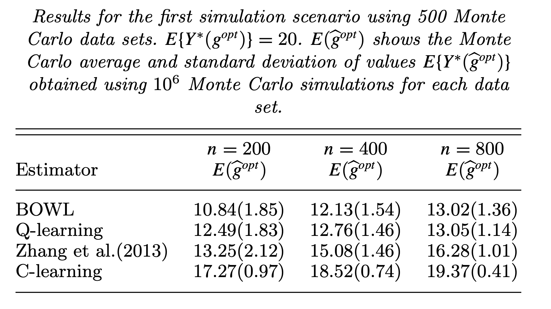
Figure 3: Simulation results from other literatures with the same simlation setting

Case 2: Two stage rewards

In Case 1, intermediate rewards are set to be 0, while in Case 2, these rewards will be taken into consideration, or in other words, the weights are now $w_{t} = 1$ rather than $w_{t} = 0, t \in {1, 2}$ in Case 1. Additionally, in Case 1 the covariates at later stages are predetermined before the trial starts, i.e., they are independent of all future interventions, which is not quite realistic. The simulation setting we adopted here is borrowed from simulation scenario 2 in Zhao et al. (2015). Specifically, there are 50 baseline covariates that are generated from normal distribution and two intermediate covariates are generated accordingly; see below. $\begin{aligned} X_{1, i} & \sim N (0, 1), i = 1, . . ., 50 \\ X_{2, 1} & \sim I [N (1.25 X_{1, 1} (2 A_{1} - 1), 1) > 0] \\ X_{2, 2} & \sim I [N (- 1.75 X_{1, 2} (2 A_{1} - 1), 1) > 0] \end{aligned}$ and the treatment assignments at stage 1 and 2 are randomly generated from ${0, 1}$ with equal probability. The outcomes at each stage are generated as follows $\begin{aligned} Y_{1} & \sim N ((1 + 1.5 X_{1, 3}) (2 A_{1} - 1), 1) \\ Y_{2} & \sim N ((Y_{1} + A_{1} + 0.5 X_{2, 1} - 0.5 X_{2, 2}) (2 A_{2} - 1), 1) \end{aligned}$

Case 2: Simulation Results

Similar to Case 1, the sample size of training varies from 100, 200, and 400, and validation set 10,000. We repeat 500 times for each scenario. The mean and variance of the estimated DTR is provided in the Table 2. The optimal mean DTR in this setting is $3.667$ . Unlike in Case 1 simulation study, T-learner yields superior performance comparing to S- and X-learner. Meanwhile, we provide the simulation results in Zhao et al. (2015) for a direct comparison; see scenario 2 in Figure 4. We can find the proposed meta-learner methods perform consistently well especially T-learner under this setting. In addition, the scenario 3 are the results of Case 1 simulation study. If considering both scenarios together, meta-learners’ performance is quite robust across all settings.

Table 2: Case 2: Results of average and stadard deviation of optimal overall outcomes from 500 Monte Carlo datasets
	n = 100	n = 200	n = 400
S-learner	2.933 (0.497)	3.081 (0.17)	3.241 (0.106)
T-learner	3.039 (0.084)	3.184 (0.077)	3.384 (0.087)
X-learner	3.006 (0.067)	3.104 (0.078)	3.377 (0.102)

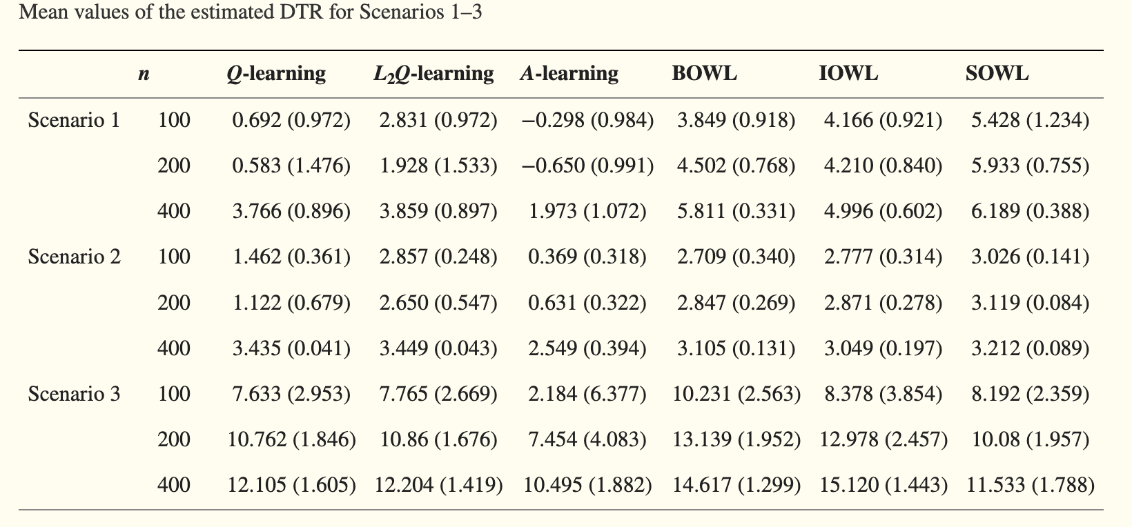
Figure 4: Simulation results for Case 1 (Scenario 3) and Case 2 (Scenario 2) from Zhao (2015)

Discussions

Multi-armed Experiment

In our previous discussions, we merely focus on scenarios with only two treatment options. When there are more than two arms, Q-learning approaches can easily be extended in most cases, it just has more Q-functions at each stage corresponding to each arm, but the value function is still well-defined and readily obtainable. However, most A-learning methods are not straightforward under multi-armed settings. The main reason is, the target quantity, the treatment effect or contrast function, need to be carefully tailored. For example, one potential way of adjustment for A-learning methods is to work on a one-versus-rest schema, or focus on pairwise comparisons between any two arms, i.e., one-versus-one schema.

These conclusions are also true for meta-learners. S- and T-learner method can easily deal with multiple-treatment scenarios but for X-learner, careful adjustments are required.

Non-randomized Design

In general, there are two sources of confounding in DTR, one comes from the unobserved influential covariates, and the other comes from past treatment assignments. For the first one, we can eliminate the impact of unobserved confounders through randomization. The second one is handled by the optimization structure introduced in Method section. When randomization is no longer achievable, we lose the control of unobserved confounding factors, and thus, to make valid inference, we need assumptions like unconfoundedness and overlapping.

Technically, propensity score will play a more important role in non-randomized studies especially for A-learning approaches, as it could provide additional security to the model misspecification, known as double robustness, along with the outcome models. Notably, for Q-learning methods, propensity score is not involved a lot. Though lose doubly robust property, Q-learning methods can achieve better approximation of outcome models, like S- and T-learner methods with powerful base learner. More importantly, in practice, when the treatment numbers are large, estimating propensity score is problematic because overlapping assumption can easily be violated. Since propensity score can have extreme values in these cases, the estimators involved propensity score might be impaired as well.

See Appendix for an example of using metaDTR package to learn the optimal DTR from a simulated observational, multi-armed, multi-stage study.

VS Reinforcement Learning

Clearly, the whole idea of seeking optimal DTR is parallel to reinforcement learning. The key is all about balancing the short-term and long-term returns to reach the optimal rewards eventually. There are some slight differences in notation/terminology though. We know the key elements of reinforcement learning includes: a set of environment and agent states, $S$ , which is history information $H$ in this work; a set of actions, $A$ , which is equivalent to treatment assignment $A$ in this work; reward after receiving action, $R$ , which is the outcome $Y$ here; the goal is to learn policy, $π (s) = Pr (a_{t} = 1 ∣ s_{t} = s)$ , which is denoted by $g_{t} (h_{t})$ . And we also have similar idea in construction of $Q ()$ and $V ()$ functions. However, the main difference is in SMART or sequential observational study, it’s a finite-decision problem with extremely small number of decisions to make, if compared with problems in reinforcement learning world. This leads to very different way to solve the problem. In DTR seeking, we do not need to know the transition probability of states, i.e., we do not need to consider the environment’s interactions; and we can use back deduction to solve the problem given finite and limited stages.

References

Bellman, R. (1966), “Dynamic programming,” Science, American Association for the Advancement of Science, 153, 34–37.

Blatt, D., Murphy, S. A., and Zhu, J. (2004), “A-learning for approximate planning,” Ann Arbor, Citeseer, 1001, 48109–2122.

Chakraborty, B., and Murphy, S. A. (2014), “Dynamic treatment regimes,” Annual review of statistics and its application, NIH Public Access, 1, 447.

Chipman, H. A., George, E. I., and McCulloch, R. E. (1998), “Bayesian CART model search,” Journal of the American Statistical Association, Taylor & Francis, 93, 935–948.

Chipman, H. A., George, E. I., and McCulloch, R. E. (2002), “Bayesian treed models,” Machine Learning, Springer, 48, 299–320.

Chipman, H. A., George, E. I., McCulloch, R. E., and others (2010), “BART: Bayesian additive regression trees,” The Annals of Applied Statistics, Institute of Mathematical Statistics, 4, 266–298.

Dorie, V., Chipman, H., McCulloch, R., Dadgar, A., Team, R. C., Draheim, G. U., Bosmans, M., Tournayre, C., Petch, M., Lucena Valle, R. de, and others (2022), “Package ‘dbarts’.”

Künzel, S. R., Sekhon, J. S., Bickel, P. J., and Yu, B. (2019), “Metalearners for estimating heterogeneous treatment effects using machine learning,” Proceedings of the National Academy of Sciences, National Acad Sciences, 116, 4156–4165.

Laber, E. B., Lizotte, D. J., Qian, M., Pelham, W. E., and Murphy, S. A. (2014), “Dynamic treatment regimes: Technical challenges and applications,” Electronic journal of statistics, NIH Public Access, 8, 1225.

Lavori, P. W., and Dawson, R. (2000), “A design for testing clinical strategies: Biased adaptive within-subject randomization,” Journal of the Royal Statistical Society: Series A (Statistics in Society), Wiley Online Library, 163, 29–38.

Moodie, E. E., Richardson, T. S., and Stephens, D. A. (2007), “Demystifying optimal dynamic treatment regimes,” Biometrics, Wiley Online Library, 63, 447–455.

Murphy, S. A. (2003), “Optimal dynamic treatment regimes,” Journal of the Royal Statistical Society: Series B (Statistical Methodology), Wiley Online Library, 65, 331–355.

Murphy, S. A. (2005b), “A generalization error for q-learning,” Journal of Machine Learning Research, 6, 1073–1097.

Murphy, S. A. (2005a), “An experimental design for the development of adaptive treatment strategies,” Statistics in medicine, Wiley Online Library, 24, 1455–1481.

Murphy, S. A., Laan, M. J. van der, Robins, J. M., and Group, C. P. P. R. (2001), “Marginal mean models for dynamic regimes,” Journal of the American Statistical Association, Taylor & Francis, 96, 1410–1423.

Nahum-Shani, I., Qian, M., Almirall, D., Pelham, W. E., Gnagy, B., Fabiano, G. A., Waxmonsky, J. G., Yu, J., and Murphy, S. A. (2012), “Experimental design and primary data analysis methods for comparing adaptive interventions.” Psychological methods, American Psychological Association, 17, 457.

Robins, J. M. (2004), “Optimal structural nested models for optimal sequential decisions,” in Proceedings of the second seattle symposium in biostatistics, Springer, pp. 189–326.

Schulte, P. J., Tsiatis, A. A., Laber, E. B., and Davidian, M. (2014), “Q-and a-learning methods for estimating optimal dynamic treatment regimes,” Statistical science: a review journal of the Institute of Mathematical Statistics, NIH Public Access, 29, 640.

Shi, C., Fan, A., Song, R., and Lu, W. (2018), “High-dimensional a-learning for optimal dynamic treatment regimes,” Annals of statistics, NIH Public Access, 46, 925.

Wagner, E. H., Austin, B. T., Davis, C., Hindmarsh, M., Schaefer, J., and Bonomi, A. (2001), “Improving chronic illness care: Translating evidence into action,” Health affairs, Project HOPE-The People-to-People Health Foundation, Inc., 20, 64–78.

Zhang, B., Tsiatis, A. A., Laber, E. B., and Davidian, M. (2013), “Robust estimation of optimal dynamic treatment regimes for sequential treatment decisions,” Biometrika, Oxford University Press, 100, 681–694.

Zhang, B., and Zhang, M. (2018), “C-learning: A new classification framework to estimate optimal dynamic treatment regimes,” Biometrics, Wiley Online Library, 74, 891–899.

Zhao, Y.-Q., Zeng, D., Laber, E. B., and Kosorok, M. R. (2015), “New statistical learning methods for estimating optimal dynamic treatment regimes,” Journal of the American Statistical Association, Taylor & Francis, 110, 583–598.

Appendix

Here we consider a simulation setting that is way more complicated than the cases used in simulation section. It is an observational, multi-armed, and multi-stage study. Consider a two-stage study that at first stage, subjects only take treatment $\in {0, 1}$ , but in second stage, subject’s treatment assignment will be based on the previous outcomes, i.e., if original control effect ( $A = 0$ ) is not satisfying, subject will move to treatment arms ( $A = 1$ ); else, they stay in control arm. If previous treatment effect ( $A = 1$ ) is good, they have chance to further escalate to higher dose level ( $A \in {2, 3}$ ); else, switch to control arm. See detailed simulation settings below: $\begin{aligned} X_{1, i} & \sim N (0, 1), i = 1, . . ., 50 \\ X_{2, 1} & \sim I [N (1.25 X_{1, 1} (2 A_{1} - 1) + X_{1, 2}, 1) > 0] \\ X_{2, 2} & \sim I [N (- 1.75 X_{1, 2} (2 A_{1} - 1) + X_{1, 3}, 1) > 0] \\ X_{2, j} & \sim N (0, 1), i = 3, . . ., 10 \end{aligned}$ $\begin{aligned} logit (Pr (A_{1} = 0)) & = X_{1, 1} + X_{1, 2} X_{1, 3} + X_{1, 4}^{2} / 3 \\ Pr (A_{2} = 0) & = \frac{(1 - A_{1}) Y_{1}^{2} + X_{2, 1}}{C} \\ Pr (A_{2} = 1) & = \frac{A_{1} Y_{1}^{2} + X_{2, 1}}{C} \\ Pr (A_{2} = 2) & = \frac{A_{1} Y_{1}^{2} + X_{2, 1}}{C} \\ Pr (A_{2} = 3) & = \frac{A_{1} Y_{1}^{2} / 6 + X_{2, 1}}{C} \\ C & = \sum_{j = 0}^{3} Pr (A_{2} = j) \end{aligned}$

$\begin{aligned} Y_{1} & \sim N ((1 + X_{1, 3} - X_{1, 2}) (2 A_{1} - 1) + X_{1, 5}, 1) \\ Y_{2} & \sim N ((Y_{1} + A_{1} + 0.5 X_{2, 1} - 0.5 X_{2, 2}) A_{2} + X_{1, 5}, 1) \end{aligned}$ The code of applying package metaDTR is provided below:

## solve by package metaDTR:
X = list(X1.tr, X2.tr)
A = list(as.factor(A1.tr), as.factor(A2.tr))
Y = list(Y1.tr, Y2.tr)
DTRs = learnDTR(X = X,
                A = A,
                Y = Y,
                weights = rep(1, length(X)),
                baseLearner  = c("BART"),
                metaLearners = c("S", "T"),
                include.X = 1, 
                include.A = 2, 
                include.Y = 1,
                verbose = FALSE
)
## test data at baseline
X1.te = matrix(rnorm(n.test*nX1, 0, sigma), ncol = nX1)
## make recommendations based on current info
A1.opt = recommendDTR(DTRs, X.new = X1.te)
## Y2/X2 is dependent on A1 (in practice, Y2/X2 should be observed)
Y1.te = Y1.fun(n.test, X1.te, as.numeric(A1.opt$A.opt.S$Stage.1)-1)
X2.te = X2.fun(n.test, X1.te, as.numeric(A1.opt$A.opt.S$Stage.1)-1)
## then keep updating it by providing newly observed info 
A2.opt = recommendDTR(DTRs, currentDTRs = A1.opt, 
                      X.new = X2.te, , Y.new = Y1.te)

## original rewards:
mean(Y1.tr+Y2.tr)

## [1] 1.66878

## optimized rewards (S-learner)
mean(Y.fun(X1.te, X2.te, Y1.te,
           as.numeric(A2.opt$A.opt.S$Stage.1)-1, 
           as.numeric(A2.opt$A.opt.S$Stage.2)-1))

## [1] 6.335082

## optimized rewards (T-learner)
mean(Y.fun(X1.te, X2.te, Y1.te,
           as.numeric(A2.opt$A.opt.T$Stage.1)-1, 
           as.numeric(A2.opt$A.opt.T$Stage.2)-1))

## [1] 6.106891

## distribution of optimized A1:
table(A2.opt$A.opt.T$Stage.1)

## 
##   0   1 
## 186 814

## distribution of optimized A2:
table(A2.opt$A.opt.T$Stage.2)

## 
##   0   1   2   3 
##  33  39 555 373

Clearly, optimal DTR on average yields way better rewards than original assignment that without any personalization. Also, by simulation setting we know that larger A better treatment effect, which is also well reflected in the distribution of recommended treatment assignments at both stage.

Here is another example of applying package metaDTR on simulation Case 1 data. In that case, intermediate covariates can be predetermined before the study. So the optimal DTRs can be obtained immediately from the function recommendDTR(). The results are close to what we have seen in Simulation section.

X = list(X1.tr, X2.tr, X3.tr)
A = list(as.factor(A.tr[,1]), as.factor(A.tr[,2]), as.factor(A.tr[,3]))
Y = list(0, 0, Y.tr)
## training
DTRs = learnDTR(X = X,
                A = A,
                Y = Y,
                weights = rep(1, length(X)),
                baseLearner  = c("BART"),
                metaLearners = c("S", "T"),
                include.X = 1, 
                include.A = 2, 
                include.Y = 0,
                verbose = FALSE
)
## estimate optimal DTR for testing data:
optDTR <- recommendDTR(DTRs, currentDTRs = NULL,
                       X.new = list(X1.te, X2.te, X3.te)) 
## S-learner results:
Y.eva.S = y.fun(X1.te, X2.te, X3.te, 
                matrix(as.numeric(unlist(optDTR$A.opt.S))-1, ncol = 3, byrow = F))
mean(Y.eva.S)

## [1] 19.61549

## T-learner results:
Y.eva.T = y.fun(X1.te, X2.te, X3.te, 
                matrix(as.numeric(unlist(optDTR$A.opt.T))-1, ncol = 3, byrow = F))
mean(Y.eva.T)

## [1] 19.44285