Positive-and-Unlabeled Learning

Introduction

Positive and unlabeled learning, or positive-unlabeled (PU) learning, refers to the binary classification problem where only positive labels are observed and the rest are unlabeled. Since unlabeled part of data consists of both positive and negative instances, naively treating them as negative and performing a standard classification learning algorithm will underestimate the probability of being positive (Ward et al. 2009; Peng Yang et al. 2012). Without providing negative instances in the training set, however, will prevent the direct use of well-developed supervised classification methods. To break through this dilemma, dozens of PU learning algorithms have been proposed in the past two decades.

One way to bypass the lack of negative instances is to disregard the unlabeled part and only learn from positive instances. Given this underlying idea is similar to one-class classification problem, which is designed do classification when the negative instances are absent, poorly sampled, or not well defined (Khan and Madden 2014), many existing one-class learning algorithms could be easily formulated to PU learning (Pengyi Yang, Liu, and Yang 2017), such as Positive Naive Bayesian (PNB) (Wang et al. 2006; Calvo, Larrañaga, and Lozano 2007), one-class SVM (Joachims 1999; De Bie et al. 2007; W. Li, Guo, and Elkan 2010), and one-class KNN (Munroe and Madden 2005). However, since unlabeled instances are not used during the training step, it may not be competitive to those algorithms which could effectively utilize information from both positive and unlabeled instances.

To better utilize the unlabeled instances, one class of algorithms adopt a heuristic two-step strategy (Manevitz and Yousef 2001; Yu, Han, and Chang 2002; Liu et al. 2002, 2003; X. Li and Liu 2003; Peng Yang et al. 2012). In the first step, instances that are likely to have negative labels are identified by certain similarity, or distance metrics. In the second step, a classifier is developed based on the positive instances, quasi-negative instances detected in the first step, and remaining unlabeled instances. Alternatively, another branch of methods let positive and unlabeled instances share different weights in the loss function and/or classification model to account for the asymmetric nature of PU learning problem. Many existing classification algorithms that are able to incorporate weights have been studied, such as naive Bayes (Nigam et al. 2000), biased SVM (Liu et al. 2003), and biased logistic model (Lee and Liu 2003). One potential drawback of the aforementioned methods is they either explicitly or implicitly rely on the assumption that data are generated from a mixture model (Nigam et al. 2000). Hence, they are more appropriate for deterministic scheme but not probabilistic scheme, following the nomenclature proposed by Song et al. (Song and Raskutti 2019).

Meanwhile, a more theoretical viewpoint of PU learning has been developed by putting it into a case-control framework (Ward et al. 2009), given the fact that the way of sampling is not the same for positive set and unlabeled set. In positive set, only instances with positive true label are sampled, which are called cases. Unlabeled set, on the other hand, is a complete random sampling from the population, which serves as controls. Under this framework, Ward et al. are able to estimate the underlying positive-negative logistic model from observed positive-unlabeled data by expectation-maximization (EM) algorithm (Dempster, Laird, and Rubin 1977). Recently, Song et al. (Song and Raskutti 2019) extend this method with penalty terms to accomplish variable selection, and convergence is guaranteed. Denote $x$ as covariates, $y$ as unobserved true label, and $z$ as observed label where unlabeled instances are treated negative. The main flaw of this method is we need to know the population prevalence $Pr(y=1)$, which is almost impossible in practical application, otherwise it is not identifiable with observed positive and unlabeled instances (Ward et al. 2009). Slightly different from case-control modeling, Elkan et al. and Scott et al. (Elkan and Noto 2008; Scott and Blanchard 2009) consider a single-training-set scenario that all instances are sampled from a joint distribution of $(x,y,z)$ but only $(x,z)$ is recorded. The estimation of population prevalence is obvious under this setting, but an unrealistic noiseless assumption $P(y=1\mid x)=1$ is required. Therefore, they provide a weighting approach that could get rid of this assumption. However, this approach can be viewed as a one-step iteration of Ward’s EM algorithm (Song and Raskutti 2019).

Recently, researchers incorporate bagging (Breiman 1996) idea into the PU learning to generate final classifier by assembling multiple PU classifiers estimated from bootstrap sampling (Mordelet and Vert 2011; Mordelet and Vert 2014; Claesen et al. 2015; Pengyi Yang et al. 2016). This approach takes advantage of bagging feature to reduce noise from modeling directly with unlabeled instances and obtain more stable predictions. Rather than using unanimous probability to sample, AdaSample (Pengyi Yang et al. 2018), a more boosting-like algorithm, applies different sampling probability at each step, and the probability is calculated from PU model estimated in the previous iteration. The performance of the adopted PU classifier for the bootstrap sample is of great importance to the success of this set of methods.

PUwrapper (basic idea)

The PUwrapper provides a general framework that could apply to any traditional supervised learning algorithm but still make them work for the Positive-Unlabeled dataset.

In positive-only data scene, there are two fundamental setup:

• Condition 1. Positive instances are completely random selection from positive population;
• Condition 2. The unlabeled instances are a random sampling from the population.

As the observed dataset is not a random sample from the population but a random sample for either the positive or the unlabeled, it satisfies the case-control framework. But among the unlabeled, there is a mixture of true positive and negative instances which makes it hard to directly adopt traditional methods upon this case-control problem.

Since only part of $y$ is observed, PU problem can be viewed as a missing data problem and one commonly used method for the missing data problem is EM algorithm (Dempster, Laird, and Rubin 1977). In the following sections, we will first introduce existing EM algorithm designed for PU problem as well as the basic idea of PUwrapper.

• Observed likelihood: $$L^{obs}(\theta \mid x,z,s=1)=\prod _i{P}_{\theta }(z_i=1\mid s_i=1,x_i{)}^{z_i}(1-P_{\theta }(z_i=1\mid s_i=1,x_i){)}^{1-z_i}$$ which relevant to $P_{\theta }(z_i=1\mid s_i=1,x_i)$ but not the desired one $P_{\theta }(y_i=1\mid x_i)$. An adjustment could be make upon the observed likelihood function to target on $P_{\theta }(y_i=1\mid x_i)$ but that is hard to solve (Ward et al. 2009). Hence, an EM algorithm is proposed because it is a simple missing label problem and could be easier to work with full likelihood.

• Full likelihood: $$L^{full}(\theta \mid x,y,z,s=1)\propto \prod _i{P}_{\theta }(y_i=1\mid s_i=1,x_i{)}^{y_i}{P}_{\theta }(y_i=0\mid s_i=1,x_i{)}^{1-y_i}$$

• EM algorithm (adjusted): maximize the observed likelihood by iteratively maximize the full likelihood conditioning on the observed data and estimated parameters. Here let $$\begin{array}{rl}{f}_{\theta }^{\ast }(x)& :=P_{\theta }(y=1\mid x,s=1);\\ f_{\theta }(x)& :=P_{\theta }(y=1\mid x).\end{array}$$

• E-step: $$\begin{array}{rl}Q(\theta \mid {\theta }^{(k)})& =E[{\ell }^{full}(\theta \mid x,y,z,s=1)\mid x,z,s=1,{\theta }^{(k)}]\\ & =\sum _i\{E[y_i\mid z_i,x_i,s_i=1,{\theta }^{(k)}]\log f_{\theta }^{\ast }(x_i)+(1-E[y_i\mid z_i,x_i,s_i=1,{\theta }^{(k)}])\log (1-f_{\theta }^{\ast }(x_i))\}\end{array}$$ where $E[y_i\mid z_i,x_i,s_i=1,{\theta }^{(k)}]=f_{{\theta }^{(k)}}(x_i{)}^{(1-z_i)}$.

• M-step: In M-step, we maximize the expectation of full log-likelihood described in E-step $${\theta }^{(k+1)}=\arg \underset{\theta }{max}Q(\theta \mid {\theta }^{(k)}).$$

• Mapping: We add an additional step here to make it work like a wrapper that are free of the specification of functional structure of $f_{\theta }^{\ast }(x)$ and $f_{\theta }(x)$. After optimizing in M-step, we will obtain ${\hat{\theta }}^{(k+1)}$ as well as $f_{{\hat{\theta }}^{(k+1)}}^{\ast }(x)$, but if using ${\hat{\theta }}^{(k+1)}$ means we need to know the functional structure of $f_{\theta }(x)$. Instead, we could directly find the relationship between $f_{\theta }(x)$ and $f_{\theta }^{\ast }(x)$: $$f_{\theta }(x)=\frac{(c-1)f_{\theta }^{\ast }(x)}{c-f_{\theta }^{\ast }(x)}$$ where $$c=\frac{Pr(y=1\mid s=1)}{Pr(z=1\mid s=1)}.$$

• How to achieve c?

In formula $c=\frac{Pr(y=1\mid s=1)}{Pr(z=1\mid s=1)}$, $Pr(z=1\mid s=1)$ is observed but $Pr(y=1\mid s=1)$ is relevant to population prevalence $\pi =P(y=1)$ which is unknown. In most literature, $\pi$ is assumed to be known. But in real application, $\pi$ is always infeasible, and thus hinter the application of their methods. However, noticing that $$\begin{array}{rl}E(y\mid s=1)& =E_x[E(y\mid s=1,x)]\\ & =\frac{1}{n}\sum _{i}Pr(y_i=1\mid s_i=1,x_i)\\ & =\frac{1}{n}\sum _i{f}_{\theta }^{\ast }(x_i),\end{array}$$ we could replace the unknown $E(y\mid s=1)$ by the empirical value. That is $$f_{{\theta }^{(k+1)}}(x)=\frac{(\frac{1}{n}\sum _i{f}_{{\hat{\theta }}^{(k+1)}}^{\ast }(x_i)-1)f_{{\hat{\theta }}^{(k+1)}}^{\ast }(x_i)}{\frac{1}{n}\sum _i{f}_{{\hat{\theta }}^{(k+1)}}^{\ast }(x_i)-f_{{\hat{\theta }}^{(k+1)}}^{\ast }(x_i)}.$$

• How to do variable selection during EM

If we want to accomplish variable selection during the EM algorithm, the objective function at M-step is adjusted to the following $${\theta }^{(k+1)}=\arg \underset{\theta }{max}Q(\theta \mid {\theta }^{(k)})+\lambda J(\theta ).$$ Imputation-regularized optimization (IRO) developed by Liang et al. (2018) propose a general idea of handling missing data (in variables not outcomes) in high dimensional data. PULasso (Song and Raskutti 2019) adopts quadratic majorization for M-step (QM-EM) which mainly targets on computational efficacy.

Basically, as a wrapper, we do not need to know specific value of ${\theta }^{(k+1)}$. Instead, what a wrapper needs is simply $f_{\theta }^{\ast }(x_i)$. So variable selection, if necessary, should be embedded in the wrapped algorithm. For example, PLR or Reinforced Learning Tree (RLT) if wrapped, are able to select important variables.

• Unbalanced scenarios (observation unbalancedness and population unbalancedness) This is not something we are interested for a wrapper. If necessary, we could start with rewriting c as $$c=1+Pr(y=1\mid z=0,s=1)\frac{Pr(z=0\mid s=1)}{Pr(z=1\mid s=1)}$$ and the unbalancedness is explicitly expressed in second term. Specifically, population unbalancedness is expressed by $Pr(y=1\mid z=0,s=1)$, since $Pr(y=1\mid z=0,s=1)=Pr(y=1)$ under Condition 2, and $\frac{P(z=0\mid s=1)}{P(z=1\mid s=1)}$ is a measure of observation unbalancedness.

• How to find out the optimal cutoff without knowing the true $\pi$

We are able to generate a sequence of estimated probability for each unlabeled instance, even though the probability itself is biased, the order is maintained (shown by ROC curve). For application purpose, sometimes we need to provide a clear category for instances which could be a problem when true $\pi$ is not provided. One way is to estimate $\pi$ from estimated c, which is obtained at convergence of the algorithm. However, we should also be aware of the potential biasness of such estimator, since $\pi$ is not identifiable.

Illustration via Simple Simulation Studies

In the first simulation study, we compare the outcomes from knowing true $\pi$ to those using estimated $\pi$ under a simplified setting, i.e., $logit(Pr(y=1))=1.2X+\epsilon$. We display the estimated probabilities against $X$ in Figure 1 (a), (b).

Based on the results, there are several comments:

• Biased $\pi$ (equivalently, $c$) leads to biased estimations of probabilities
• Using estimated $c$ seems to be a valid solution
• Initial value to start EM algorithm does not matter a lot
• True $c$ has better convergence rate than using estimated $c$ at each step

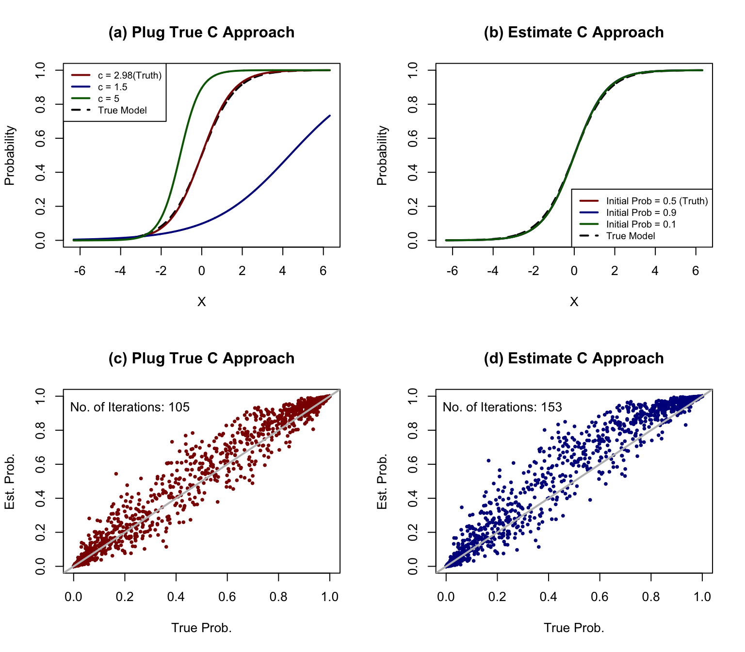
Figure 1: Simple examples of Wald’s method and the proposed improved method with estimated c. Panel (a) and (b): univariate model $logit(Pr(y=1))=1.2X$; Panel (c) and (d): multivariate model $logit(Pr(y=1))=-1+2X_1+4X_2-X_3-2X_4+X_5$, and we know the true model during fitting.

In second simulation study, we wrap two basic supervised learning algorithms: random forests (RF) and penalized logistic regression (PLR). At the meantime, we would like to conduct variable selection during the process. For PLR, we adopt LASSO at each EM iteration, while for RF, we use variable importance score as the weights. We generate 100 variables where only 5 of them are related to the outcome. In other words, the rest of them are purely noise. In Figure 2, we display the results based on PUwrapper, and the selected variables, or variable importances are given in panel (c) and (f).

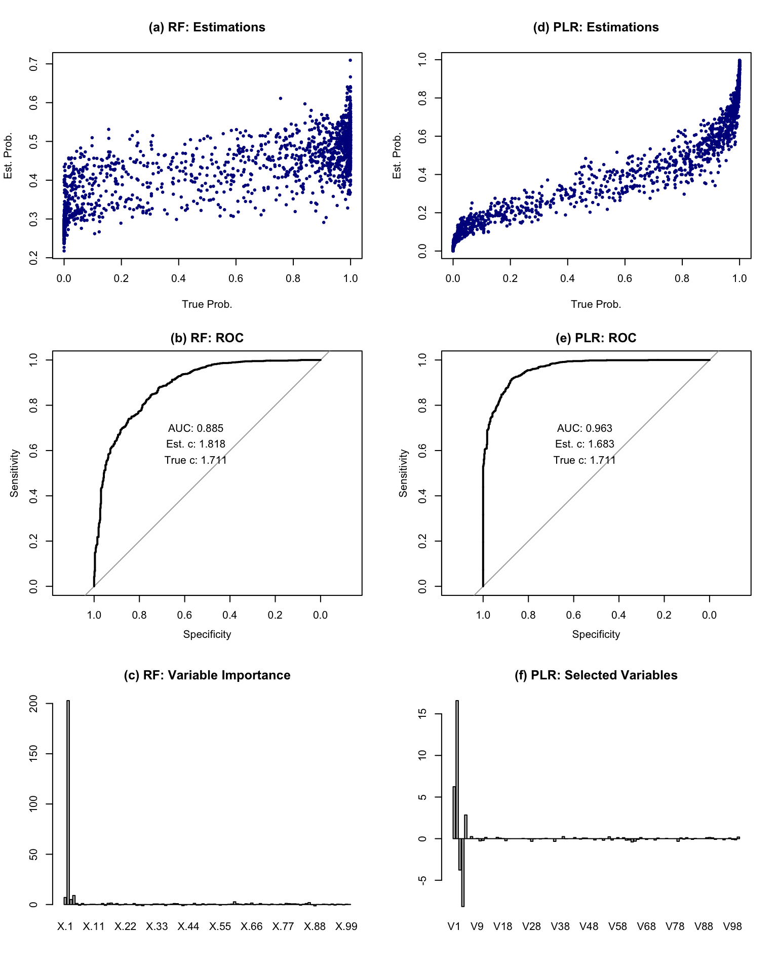
Figure 2: Simple examples of PUwrapper. Panel (a) and (b): Random Forests; Panel (c) and (d): Penalized Logistic Regression. The baseline model is $logit(Pr(y=1))=-1+2X_1+4X_2-X_3-2X_4+X_5$ with a total of 100 variables simulated. The size of simulated sample is 1600 and 600 of them are labeled as 1.