The need for causal inference arises in many different fields. Economists want to quantify the causal effects of interest rate cut on the economy. Trade policy makers want to know whether increased tariff causes changes in trade deficit. Healthcare providers want to assess whether a therapy causes changes in specific patient outcomes. Conceptually, causal inference is all about a question of ‘what if’. People can ask themself what if I took chemotherapy rather than radiation to treat my cancer, would I get better now? Or what if I went to graduate school rather than entering the job market after graduation, would I have a better career prospect? The economists can be curious about what if the Federal Reserve raised the interest rate by 50bp rather than 25bp, would the inflation rate be better controlled? The most straightforward way to answer those questions is, if we know what will happen for any of these actions in advance, we of course can choose the one benefits our goal the most. This leads to the Potential Outcome Framework that we will discuss in the next section.
Potential outcome framework, or Rubin-Neyman potential outcome framework (Donald B. Rubin 1974; Neyman 1923; Imbens and Rubin 2015), is the most canonical framework for causal inference studies. Suppose the treatment has binary levels, denoted as
To make the estimation of causal effect feasible, we have to make several assumptions:
Assumption 1. Stable Unit Treatment Value Assumption (SUTVA) (Donald B. Rubin 1980)
1) Treatment applied to one unit does not affect the outcome for other units (No Interference)
2) There is no hidden variation, for example, different forms or versions of each treatment level, for a single treatment (Consistency)
Assumption 2. Unconfoundedness/Ignorability/Strongly Ignorable Treatment Assignment (SITA)
Assumption 3. Common Support/Positivity
In the following sections, we will discuss how to estimate of the individual or sample average treatment effects under this potential outcome framework with these assumptions.
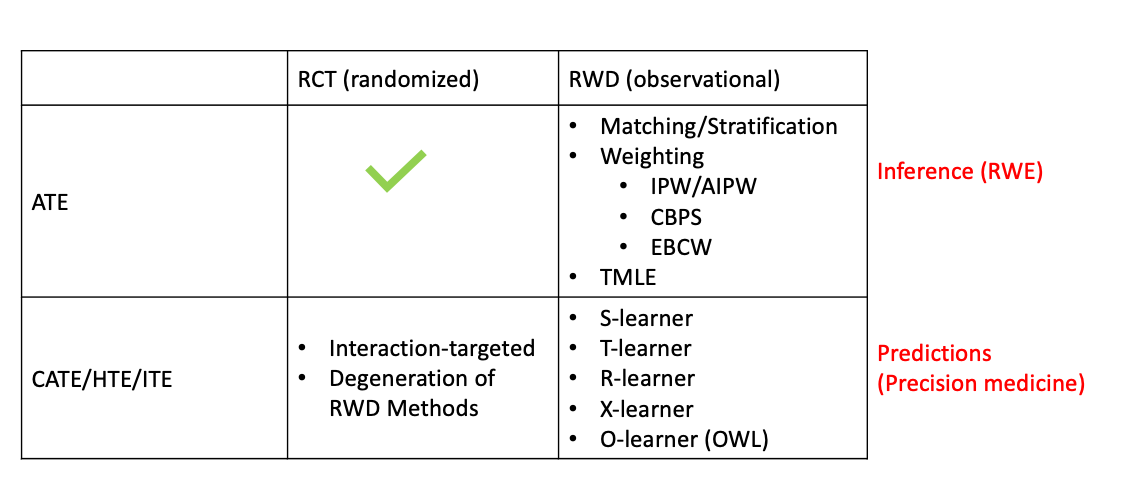
In general, most research on causal inference either studies the population-wise treatment effect, i.e., the average treatment effect (ATE), or the subject-level/individual treatment effect (ITE), i.e., the conditional treatment effect (CATE), which is exchangeable to heterogenuous treatment effect (HTE).
Basically, the observations can be either from randomized experiments, like randomized controlled trial (RCT), or observational studies, so-called real world data (RWD). With different observations, the estimation methods can be very different.
Briefly speaking, the ATE can be easily obtained via well-designed RCTs or A/B tests (we will see why in section Average Treatment Effect). That’s how pharmaceutical/biotech companies evaluate their drug effectiveness. In recent years, a big trend in drug development which is supported by FDA is to use RWD and real world evidence (RWE) to support as well as speed-up the regulatory approval. Since RWD is obervational rather than randomized controlled, a sizable methods are proposed including Matching (Rosenbaum and Rubin 1983; Austin 2014), Subclassification (Rosenbaum and Rubin 1984), Weighting (Hirano, Imbens, and Ridder 2003; Austin 2011; Austin and Stuart 2015), Regression (Donald B. Rubin 1979; D. B. Rubin 1985; Hahn 1998; Gutman and Rubin 2013), or a mixture of them (Bang and Robins 2005; Van Der Laan and Rubin 2006).
Another heat topic in causal inference is about the estimation of CATE/HTE/ITE from observational studies. This is usually tough because given the noise of observational studies and subject-level estimation, the estimates can have large variance. Various of methods have been proposed including but not limited to causal boosting (Powers et al. 2018), causal forests (Athey and Imbens 2016), individual-treatment-rule-based methods that mostly involves outcome weighted learning (OWL) (Qian and Murphy 2011; Zhao et al. 2012; X. Zhou et al. 2017; Qi et al. 2020), and several meta-learners, such as X-learner (Künzel et al. 2019) and R-learner (Nie and Wager 2020). These methods can be easily degenerated to study the CATE/HTE/ITE in randomized trials by replacing the estimated propensity scores to fixed numbers.
Different scientific questions leads to the estimation of different causal estimands. As aforementioned, ATE is basically about assessing the population/sub-population treatment effect which is the key focus for the drug companies. On the other hand, CATE is more about individual-level treatment effect, so it can be used to do precision medicine or personalized recommendations. Here is a list of the acronym of some commonly used causal estimands:
ATE can be observed from well-designed randomized controlled trial (RCT) directly, which reveals the population-wise treatment effect.
The essence here is the randomization eliminates all the confounding effects, or in other words, the Unconfoundedness and Positivity assumptions holds automatically under randomized controlled experiments.
Remark
Another commonly used causal estimand is average treatment effect for the treated (ATT), which focus on the population receive the treatment
Propensity score (PS) (Rosenbaum and Rubin 1983) is defined as the conditional probability of receiving a treatment given pre-treatment covariates
Though Matching is also a very popular approach in ATE estimation, here we discuss Weighting in details.
The very beginning idea of estimating ATE (under the Assumption 1, 2 and 3) by first finding pairs of observations with covariates close enough to each other in two arms, and then average them out:
The matching idea is finally ruled by the milestone work from Rosenbaum and Rubin (1983) who demonstrated that only matching by propensity score is good enough, because
It can be shown that (Proof in Appendix)
J. M. Robins, Rotnitzky, and Zhao (1995) augmented the IPW by a weighted average of the outcome model
The very nature of weighting is it helps to make sure the confounding covariates distribution between the observed two arms are balanced. If covariate balancing is guaranteed, then the observed data can mimic the randomized trial data and the treatment effect can be directly obtained from observations. Imai and Ratkovic (2014) propose to directly target on the covariate balancing instead of weighting. So they developed a Covariate Balancing Propensity Score (CBPS) method which is a propensity score estimating method that yields the PSs improve the covariate balancing.
The core idea of CBPS is fit a logistic PS model–maximize the likelihood function–subject to covariate balancing constraints. Specifically, the logistic PS model looks like
CBPS is just one of the Covariate-Balancing-type method to obtain the weights. There are many other methods following this idea (Hainmueller 2012; Chan, Yam, and Zhang 2016; Pirracchio and Carone 2018; Huling and Mak 2020) but will not be introduced here.
Another estimator that is receiving more attention for ATE estimation is the targeted maximum likelihood estimator (TMLE) (Van Der Laan and Rubin 2006), which also enjoys the double robustness as AIPW along with other desired features like efficient and aysmptotically linear (allows for construction of valid Wald-type confidence intervals). Either
TMLE is a two-stage procedure with the first stage to obtain an initial estimate of response surface/conditional mean response
After introducing this much methods, we would like to provide a high-level picture of how and when to use these methods. Usually, there are two-step included in propensity score (PS) related methods in causal estimand estimation.
The first step is to estimate the propensity score. There are several commonly adopted branches:
In second step, we plug in the propensity score estimated from the first step for the desired estimand. The common approaches for ATE/ATT include:
Sometimes also known as Heterogeneous Treatment effect (HTE). With assumption 1, 2, and 3, it’s definition under two-arm scenario is
As discussed, the CATE estimation under randomized setting is generally a special case of those methods under observational studies. Nonetheless, we want to briefly introduce some interaction-oriented methods that are more suitable in randomized setting.
Without loss of generality, outcome
Also be aware that the covariates of
A bunch of methods are developed following this idea: Interaction trees (Su et al. 2008, 2009), GUIDE (Generalized unbiased interaction detection and estimation) (Loh 2002; Loh, He, and Man 2015), MOB (Model-Based Recursive Partitioning) (Zeileis, Hothorn, and Hornik 2008; Seibold, Zeileis, and Hothorn 2016).
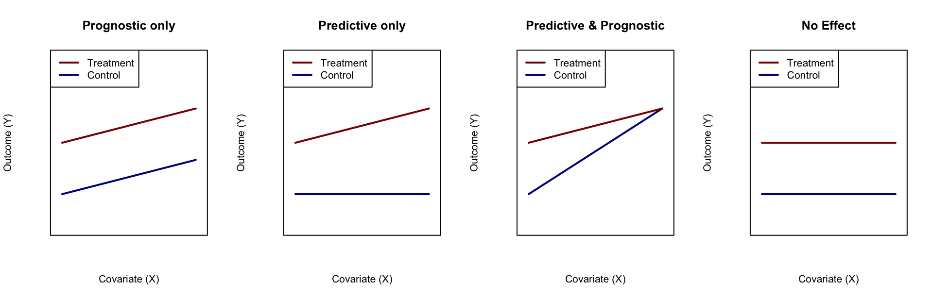
Figure 1: Illustration of predictive and diagnostic variable
Q-learning gets its name because its objective function plays a role similar to that of the Q or reward function in reinforcement learnin (Li, Wang, and Tu 2021) and is first used in estimating optimal dynamic treatment regime (Murphy 2003; J. M. Robins 2004; Schulte et al. 2014). The basic idea is focusing on the estimation of response surfaces
Estimate a joint function
Estimate response surfaces
The basic idea of advantage-learning or A-learning, is to estimate treatment effect
For a 50:50 randomized trial, we can make following transformation (Signorovitch 2007)
Notably, this method though simple and straightforward, suffers from the limitation of outcome type and the larger variance.
Observing that we only need to optimize the loss function such as (7), Tian et al. (2014) modified MOM methods by adjusting the proxy loss function a little bit
R-learner (Nie and Wager 2020) can be considered as a very special case of MCM, but it does not follow the same logic flow as MCM. It adopts the Robinson’s decomposition (Robinson 1988) to connect the CATE with the observed outcome
X-learner (Künzel et al. 2019) enjoys the simplicity of T-learner but fixes its data efficiency issue by targeting on the treatment effects rather than the response surfaces. The main procedure is the following:
Notably, when calculating
Most of the previous methods target on CATE estimation, then the optimal treatment can be found automatically by looking at the estimates. Whereas, obtaining the consistent and unbiased estimates for CATE is difficult in practice. However, if we only need to know which treatment is the optimal, we actually do not need to estimate the CATE but only the treatment assignment rule, or so-called individual-treatment-rule (ITR),
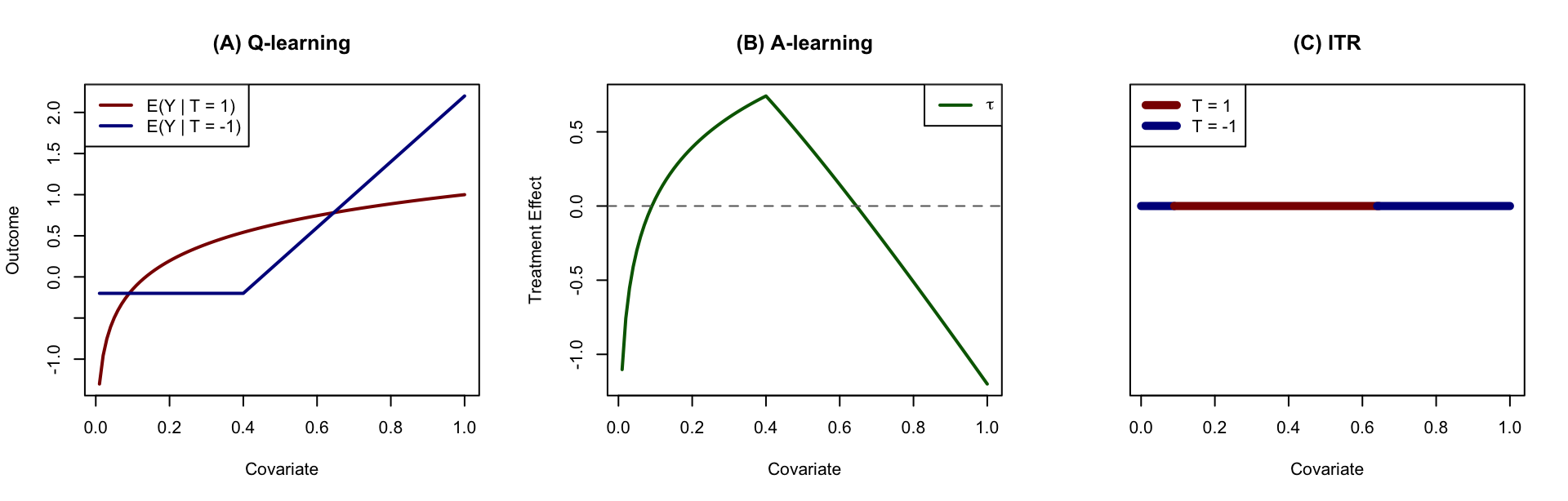
Figure 2: Illustration of causal inference approaches. (A) Q-learning aims at estimating the response surfaces of each treatment group; (B) A-learning aims at estimation of treatment effect directly; (C) ITR aims at estimation of treatment region rather than the treatment effect.
Recall the ITR is indeed a mapping from the covariate space into the treatment space
There are many tree-based methods such as virtual trees (Foster 2013), causal tree/forest (Athey and Imbens 2016; Wager and Athey 2018), causal boosting/PTO forest/causal MARS (Powers et al. 2018). Actually, most of them can be categorized as S- or T-learners on a high-level.
(For more details on CATE/HTE estimation, please refer to another post Meta-Learners)
To demonstrate that AIPW can be consistent even when propensity score is not correctly specified, we only need to focus on the general element
When propensity score is wrong, i.e.,