Idea behind OptTrialDesign
In Optimal Design Strategy, we propose a novel way to find the optimal trial design, in terms of maximizing the financial outcomes, i.e., Expected Net Revenue (ENR), but also under the regulatory requirements. We have to trade-off because in pharmaceutical companies’ position, a shorter study/trial duration leads to earlier market access which helps to maximize the profits before LOE (loss of exclusivity). On the other hand, regulatory agencies and health technology assessment (HTA) bodies wish to see more guaranteed clinical results, which usually require longer study duration. This leads to the conflicts.
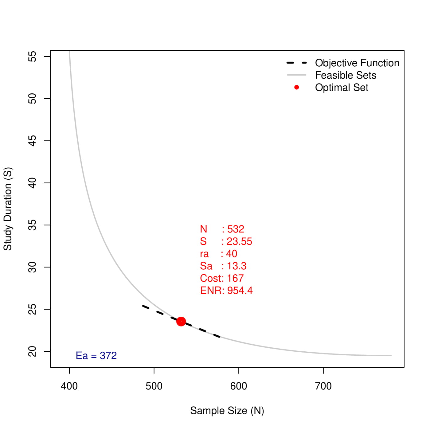
In trials with time-to-event endpoint, the trial design is still not fully determined with given target number of events. There are usually three parameters, sample size (), study duration (), and accrual rate () (or accrual duration if assuming uniform accrual rate. Here we do not consider it, and also not for trials with interim analysis, which could be extended following similar idea), and there exists infinite combinations of these three to form a trial design that could observe target number of events at the end of the study. In reality, cannot take arbitrary number as it is strongly restricted by the disease incidence/type and accrual ability of sites. Given investigators are able to provide a rough number of , or even a range of it, the degree of freedom is reduced from 3 to 2, and we are able to display the feasible sets of designs in a plane (as shown in the figure below). It is noteworthy that there is a trade-off between study duration and sample size. The larger sample size helps to accelerate the trial, and vice versa.

CAPM in Finance
Let’s take a break and turn to Capital Asset Pricing Model (CAPM) for a while. CAPM won the 1990 Nobel Memorial Prize in Economics for its contribution on pricing a portfolio analytically, and was famous for its simplicity and practical value.
In CAPM, the expected return of an asset or portfolio () can be calculated by
where is the risk-free rate (e.g., 10-year treasury rate); represents the individual risk against the market risk; and is the market risk premium. Basically, it means that in ideal situation, the riskier of an asset, the higher return is expected.
In other words, we can say that in order to find an optimal asset, we actually need to maximize the following objective function
Then, what is the feasible set? We know the expected return increases as the expected risk for an asset, but due to Law of Diminishing Marginal Utility, there should be an upper bound of the expected return (cannot go to infinity) and a lower bound of the expected risk (cannot go to 0). Usually, people believe the feasible sets is the region embraced by the parabola in the figure below. That parabola (blue curve) is called Efficient Frontier that indicates the largest (and smallest which is not of the interests) expected return at a given risk (notice the limitation of expected risk and return). The assets/portfolio not on the efficient frontier (blue circle points; Notice that there are points outside the efficient frontier simply because the efficient frontier is hypothetical, which can be violated in practice) is inefficient as you can always find another asset with the same expected risk but higher expected return on the frontier.
:max_bytes(150000):strip_icc():format(webp)/CapitalAssetPricingModelCAPM1_2-e6be6eb7968d4719872fe0bcdc9b8685.png)
Let’s rewrite the problem in the form of optimization problem as
and the objective function is actually the capital market line, the black straight line in the figure. The optimal solution is thus the tangent point (green point).
Back to Optimal Trial Design
Now let’s come back to the idea of Optimal Trial Design. Similarly, we want to maximize the ENR which can be expressed as
where is the expected sales; is the roughly the duration of exclusivity; is the total maintenance cost; is the total sample cost. The efficient frontier of feasible sets, as aforementioned, is the gray line in Figure 1. Other feasible sets above the efficient frontier are off-optimal as we can always find a better solution on the frontier with either smaller or smaller , which yield better ENR.
With exactly the same idea of CAPM, the trial design problem can be transformed into an constrained optimization problem:
and the solution is the tangent point as well (the red point).

:max_bytes(150000):strip_icc():format(webp)/CapitalAssetPricingModelCAPM1_2-e6be6eb7968d4719872fe0bcdc9b8685.png)